INFOTH Note 23: Parallel Gaussian Channels, WSS, Distributed Source Compression
Reference: T. M. Cover and J. A. Thomas, Elements of Information Theory, 2nd ed., Wiley, 2006, Ch. 9 (Gaussian Channel), especially Sec. 9.4 (Parallel Gaussian Channels). The proof sketch uses the maximum entropy theorem (Thm 8.6.5) and the entropy chain rule inequality (eq. 8.63).
23.1 Recall: AWGN Capacity
The single-use AWGN channel $Y = X + N$, $N \sim \mathcal N(0,\sigma^2)$, $X \perp\!\!\!\perp N$, has capacity
$$ C = \frac{1}{2}\log\!\left(1 + \frac{P}{\sigma^2}\right) \text{ bits per channel use}, $$- where $P$ is the per-use power constraint $E[X^2] \le P$. Communication at rate $R < C$ is achievable with $P_e^{(n)} \to 0$; rate $R > C$ is not (see Note 22).
This is also the mutual information maximizer:
$$ C = \max_{f_X:\, E[X^2]\le P} I(X;Y), \quad Y = X + N,\; X \perp\!\!\!\perp N. $$23.2 Parallel Gaussian Channel Model
Setup
Now consider $L$ parallel AWGN sub-channels used simultaneously, each has $n$ channel uses (also viewed parallel). At block index (channel use) $k \in [n]$, the $l$-th sub-channel ($l \in [L]$) satisfies
$$ Y_k^{(l)} = X_k^{(l)} + N_k^{(l)}, \quad k \in [n],\; l \in [L], $$where $N_k^{(l)} \sim \mathcal N(0, \sigma_l^2)$ are mutually independent across both $k$ and $l$, also independent from any $X_k^{(l)}$. Each sub-channel has its own noise variance $\sigma_l^2$.
The input at each block index (channel use) is a vector in $\mathbb R^L$, as well as the output. We can view the channel as $n$ channel uses and $L$ subchannels each, and the whole codeword as a matrix or a vector of $nL$ length.
Encoding and Decoding
For a message $m\in [M_n],~ M_n=2^{nR}$, we now redefine the I/O (encoding/decoding), viewing the channel as a whole with an $n$-length codeword, each element with $L$ dimensions.
$$ e_n : m \mapsto \left(\begin{bmatrix} x_1^{(1)} \\ \vdots \\ x_1^{(L)} \end{bmatrix}\!(m),\;\dots,\;\begin{bmatrix} x_n^{(1)} \\ \vdots \\ x_n^{(L)} \end{bmatrix}\!(m)\right), $$ $$ d_n : \left(\begin{bmatrix} y_1^{(1)} \\ \vdots \\ y_1^{(L)} \end{bmatrix},\;\dots,\;\begin{bmatrix} y_n^{(1)} \\ \vdots \\ y_n^{(L)} \end{bmatrix}\right) \mapsto [M_n] \cup \{*\}. $$Global Power Constraint
The total power across all sub-channels is bounded:
$$ \frac{1}{n}\sum_{k=1}^n \sum_{l=1}^L \bigl(x_k^{(l)}(m)\bigr)^2 \le P, \quad \forall\, m \in [M_n]. $$The key question is how we allocate total power $P$ among the $L$ sub-channels to maximize capacity. Note that the allocation is only for capacity computation.
23.3 Water-Filling for Capacity Allocation in Parallel Gaussian Channel Model
Statement
Theorem (Water-Filling). The capacity of the parallel Gaussian channel
$$ C = \max_{f\left(\begin{bmatrix} X^{(1)} \\ \vdots \\ X^{(L)} \end{bmatrix} \right)} I\bigl(X^{(1)},\dots,X^{(L)};\; Y^{(1)},\dots,Y^{(L)}\bigr), $$(maximum over $f$) is given by the water-filling strategy on the noise variances, where the maximum must be also subject to:
- $\sum_{l=1}^L E\bigl[(X^{(l)})^2\bigr] \le P$, where every $E\left[(X^{(l)})^2\right]$ is the power at subchannel $l$ we want to allocate;
- $Y^{(l)} \mid X = x$ are conditionally mutually independent Gaussians with mean $x^{(l)}$ and variance $\sigma_l^2$.
For the vector representation, $\bold X,\bold Y\in\R^L$, $f:\R^L\to [0,1]$,
$$ C = \max_{f(\bold X)}I(\bold X;\bold Y). $$Formal Result
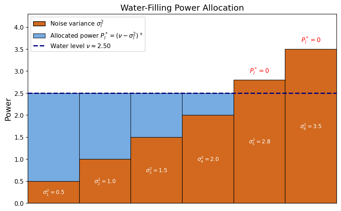
Define the water level $\nu$ as the unique value satisfying
$$ \sum_{l=1}^L (\nu - \sigma_l^2)^+ = P, \quad \text{where } z^+ := \max(z, 0). $$Then the capacity is
$$ \boxed{C = \sum_{l=1}^L \frac{1}{2}\log\!\left(\frac{\sigma_l^2 + (\nu - \sigma_l^2)^+}{\sigma_l^2}\right).} $$Equivalently, since $(\nu - \sigma_l^2)^+ = 0$ contributes $\log 1 = 0$:
$$ C = \sum_{l:\,\sigma_l^2 < \nu} \frac{1}{2}\log\frac{\nu}{\sigma_l^2}. $$The optimal power allocation to sub-channel $l$ is $P_l^* = (\nu - \sigma_l^2)^+$:
- Sub-channels with $\sigma_l^2 < \nu$ receive power $\nu - \sigma_l^2$ (the noisier, the less power).
- Sub-channels with $\sigma_l^2 \ge \nu$ are shut off ($P_l^* = 0$): too noisy to be worth using.
Water-Filling Analogy
The name comes from a physical picture: imagine a well whose floor at position $l$ has height $\sigma_l^2$. Pour $P$ units of water into the well. The water surface settles at level $\nu$, and the depth of water above position $l$ is the allocated power $P_l^* = (\nu - \sigma_l^2)^+$.
For a noise level higher over the “water level”, we simply do not allocate power.
Proof Sketch
Stage 1: Mutual Information Decomposition
The goal is to simplify $\max_f I(\bold X;\bold Y)$ to optimization about $P_1, \dots, P_L$. Since the noises $N^{(1)}, \dots, N^{(L)}$ are independent (and independent of $\bold X$):
$$ \begin{aligned} I(\bold X;\bold Y) &= h(\bold Y) - h(\bold Y \mid \bold X) \\ &= h(\bold Y) - h(N^{(1)}, N^{(2)}, \dots, N^{(L)}) \\ &= h(\bold Y) - \sum_{l=1}^L \frac{1}{2}\log(2\pi e\,\sigma_l^2). \end{aligned} $$So the optimization is equivalent to maximize $h(Y)$.
Since $\bold X\perp\!\!\!\perp \bold N$, using $E[X^{(l)} N^{(l)}] = E[X^{(l)}] E[N^{(l)}] = E[X^{(l)}]\cdot 0 = 0$,
$$ \begin{aligned} E[(Y^{(l)})^2] &= E[(X^{(l)} + N^{(l)})^2] \\ &= E[(X^{(l)})^2] + 2E[X^{(l)} N^{(l)}] + E[(N^{(l)})^2] \\ &= P_l + 2E[X^{(l)}]\,E[N^{(l)}] + \sigma_l^2 \\ &= P_l + \sigma_l^2. \end{aligned} $$Now $E[(Y^{(l)})^2] = P_l + \sigma_l^2$ where $P_l = E[(X^{(l)})^2]$.
So the only thing we can control is the input distribution (and hence $P_l$ as the second moment); the noise variances $\sigma_l^2$ are fixed. So once we fix $P_l$, the second moment of $Y^{(l)}$ is determined to be $P_l + \sigma_l^2$.
This lets us upper-bound $h(\bold Y)$.
-
By the chain rule and the fact that conditioning reduces entropy,
$$ h(\bold Y) = h(Y^{(1)}, \dots, Y^{(L)}) = h(Y^{(1)}) + \sum_{l=2}^L h(Y^{(l)} \mid Y^{(1)}, \dots, Y^{(l-1)}) \le \sum_{l=1}^L h(Y^{(l)}), $$with equality iff $Y^{(1)}, \dots, Y^{(L)}$ are independent.
-
For each $l$, we apply the maximum entropy theorem (Cover & Thomas Thm 8.6.5, scalar case), i.e. for zero-mean r.v. $Z$ with variance $E[Z^2] = \alpha$, then $h(Z) \le \frac{1}{2}\log(2\pi e\,\alpha)$, with equality iff $Z \sim \mathcal N(0, \alpha)$.
Note that Thm 8.6.5 requires zero mean. But $Y^{(l)} = X^{(l)} + N^{(l)}$ has possibly nonzero mean $E[X^{(l)}]$.
Here shows how we tackle this issue.
By translation invariance of differential entropy (See Note 9 or Cover & Thomas Thm 8.6.3), $h(Y^{(l)}) = h(Y^{(l)} - b)$ for every real constant $b$, hence $h(Y^{(l)}) = h(Y^{(l)} - E[Y^{(l)}])$.
The centered variable $Y^{(l)} - E[Y^{(l)}]$ has zero mean, whose second moment (or variance) is, by the translation invariance of variance,
$$ \begin{aligned} \mathrm{Var}(Y^{(l)} - E[(Y^{(l)})^2]) &= \mathrm{Var}(Y^{(l)}) \\ &= E[(Y^{(l)})^2] - (E[Y^{(l)}])^2 \\ &= P_l + \sigma_l^2 - (E[Y^{(l)}])^2 \\ &= P_l + \sigma_l^2 - E[X^{(l)}]^2 \\ &\le P_l + \sigma_l^2, \end{aligned} $$with equality iff $E[X^{(l)}] = 0$.
So for a single r.v. $Y^{(l)}$,
$$ h(Y^{(l)}) \le \frac{1}{2}\log\bigl(2\pi e\,(P_l + \sigma_l^2)\bigr), $$with equality iff $E[X^{(l)}] = 0$ and $Y^{(l)}$ is Gaussian, i.e. $Y^{(l)} \sim \mathcal N(0,\, P_l + \sigma_l^2)$.
The zero-mean condition is optimal with an intuition that any nonzero $E[X^{(l)}]$ wastes power, i.e. contributes to $E[(X^{(l)})^2]$, without increasing entropy, when we need a maximum entropy under limited power.
Hence
$$ h(\bold Y) \le \sum_{l=1}^L \frac{1}{2}\log\bigl(2\pi e\,(P_l + \sigma_l^2)\bigr). $$Subtracting the fixed noise entropy by $I(\bold X;\bold Y) = h(\bold Y) - h(\bold Y \mid \bold X)$, we get
$$ I(\bold X;\bold Y) \le \sum_{l=1}^L \left[\frac{1}{2}\log\bigl(2\pi e\,(P_l + \sigma_l^2)\bigr) - \frac{1}{2}\log(2\pi e\,\sigma_l^2)\right] = \sum_{l=1}^L \frac{1}{2}\log\!\left(1 + \frac{P_l}{\sigma_l^2}\right). $$Discussion of overall equality condition for the inequality above.
We state the equality conditions for the overall (vector) case.Since from above, discussing about $\bold Y$ we have the equality condition $\forall \,l \in [L]$,
- $Y^{(l)}$ are mutually independent (equality condition in 1.), and
- each $Y^{(l)}$ is Gaussian (eq. cond. in 2.).
Since
- $Y^{(l)} = X^{(l)} + N^{(l)}$ and $N^{(l)} \sim \mathcal N(0, \sigma_l^2)$ is fixed, $Y^{(l)}$ is Gaussian iff $X^{(l)} \sim \mathcal N(0, P_l)$ (sum of two independent Gaussians is Gaussian);
- The noises are already independent of each other and of $\bold X$, making $X^{(1)}, \dots, X^{(L)}$ independent suffices to make $Y^{(1)}, \dots, Y^{(L)}$ independent.
Therefore, in terms of $f$ or $\bold X$, the upper bound (bounded by $P_1,\dots,P_L$) is achieved by choosing $X^{(1)}, \dots, X^{(L)}$ as independent Gaussians with $X^{(l)} \sim \mathcal N(0, P_l)$, and the capacity optimization reduces to choosing the power allocation $P_1, \dots, P_L$.
Stage 2: Optimization Problem
With independent Gaussian inputs, the capacity reduces to its tight upper bound:
$$ \max_{P_1, \dots, P_L} \sum_{l=1}^L \frac{1}{2}\log\!\left(1 + \frac{P_l}{\sigma_l^2}\right), \quad \text{s.t. } \sum_{l=1}^L P_l \le P,\; P_l \ge 0. $$Since $\log$ is increasing, the objective is monotonically increasing in each $P_l$. Therefore the power constraint is tight at the optimum: $\sum_l P_l = P$.
Stage 3: KKT Conditions
Rewrite as a minimization problem:
$$ \min_{P_1, \dots, P_L}\; -\sum_{l=1}^L \frac{1}{2}\log\!\left(1 + \frac{P_l}{\sigma_l^2}\right). $$The Lagrangian with multiplier $\lambda \ge 0$ for the sum constraint and $\mu_l \ge 0$ for $-P_l \le 0$:
$$ \mathcal L := -\frac{1}{2}\sum_{l=1}^L \log\!\left(1 + \frac{P_l}{\sigma_l^2}\right) + \lambda\!\left(\sum_{l=1}^L P_l - P\right) - \sum_{l=1}^L \mu_l P_l. $$The KKT conditions are:
-
Stationarity (${\partial \mathcal L \over \partial P_l} = 0$):
$$ -\frac{1}{2(\sigma_l^2 + P_l)} + \lambda - \mu_l = 0, \quad \forall\, l. $$ -
Primal feasibility: $\sum_{l=1}^L P_l \le P$, $\;P_l \ge 0$.
-
Dual feasibility: $\lambda \ge 0$, $\;\mu_l \ge 0$.
-
Complementary slackness: $\lambda\bigl(\sum_l P_l - P\bigr) = 0$, $\;\mu_l P_l = 0$.
From 1. and 4., for each $l$:
- If $P_l > 0$: then $\mu_l = 0$, so $\sigma_l^2 + P_l = \frac{1}{2\lambda}$. Setting $\nu := \frac{1}{2\lambda}$ gives $P_l = \nu - \sigma_l^2$.
- If $P_l = 0$: then $\mu_l \ge 0$ forces $\frac{1}{2(\sigma_l^2)} \le \lambda$, i.e. $\sigma_l^2 \ge \nu$.
Combining: $P_l = (\nu - \sigma_l^2)^+ = \max(\mu - \sigma_l^2, 0)$, where $\nu$ is determined by $\sum_l (\nu - \sigma_l^2)^+ = P$. $\square$
23.4 Colored Noise Channels and Szegő Theorem
The parallel Gaussian model has a finite number $L$ of sub-channels. Though in practice, a waveform channel is not only continuous-time and bandlimited (say to bandwidth $W$) following the waveform channel constraints, but also with colored (non-white) noise whose power spectral density (PSD) $S_{NN}(f)$ varies continuously with frequency.
We want the capacity of this colored noise channel. Step by step, we do these things:
- The colored noise is a continuous-time WSS random process (recall 22.3). Under WSS, the PSD is well-defined and describes the noise power at each frequency.
- Nyquist sampling converts the continuous-time process to a discrete-time WSS process, and LTI filtering explains how colored noise arises.
- Taking $n$ samples of the discrete-time noise, the covariance matrix is Toeplitz (a consequence of WSS). Eigendecomposing it gives $n$ parallel sub-channels with noise variances equal to the eigenvalues.
- Apply the water-filling theorem (23.3) to these $n$ sub-channels.
- Take $n \to \infty$: Szegő’s theorem converts the sum over eigenvalues into an integral over the PSD, yielding the continuous-frequency capacity formula.
From Continuous-Time to Discrete-Time
The physical channel has continuous-time, bandlimited noise (bandwidth $W$). By the Nyquist-Shannon sampling theorem, a signal bandlimited to $[-W, W]$ is fully characterized by its samples taken at Nyquist rate $f_s = 2W$.
By sampling (time: $t = nT_s = {n\over f_s}$) we transform the continuous-time WSS noise into a discrete-time WSS process.
Why colored noise exists in practice: LTI filtering.
Our channel model simply takes the noise PSD $S_{NN}(f)$ as given. But why is it non-flat in practice?
A linear time-invariant (LTI) system is characterized by its transfer function $H(f)$: for input with PSD $S_{\text{in}}(f)$, the output PSD is $S_{\text{out}}(f) = |H(f)|^2 \cdot S_{\text{in}}(f)$. If the underlying thermal noise is white ($S_{\text{in}}(f) = {N_0\over 2}$) but the physical channel acts as a non-flat filter, the noise arriving at the receiver has PSD $|H(f)|^2 \cdot {N_0\over 2}$, which varies with frequency. WSS is preserved under LTI filtering, so the result is still a WSS process.
Discrete-Time WSS and PSD
A discrete-time WSS process $(X_k, k \in \mathbb Z)$ has an autocorrelation function that only depends on the lag $k$ (not on $n$):
$$ R_{XX}(k) := E[X_n X_{n+k}], $$Note $R_{XX}(-k) = R_{XX}(k)$.
This is the discrete-time analogue of the continuous-time WSS definition in 22.3. The dependence solely on lag is what makes the covariance matrix of $(X_1, \dots, X_n)$ a Toeplitz matrix (entry $(i,j)$ equals $R_{XX}(i-j)$, depending only on the row-column difference). The Toeplitz structure is the prerequisite for Szegő’s theorem below.
The power spectral density (PSD) is the discrete-time Fourier transform (DTFT) of the autocorrelation:
$$ S_{XX}(\hat f) = \sum_{k \in \mathbb Z} R_{XX}(k)\, e^{-j2\pi \hat f k}, \quad \hat f \in \bigl[-\tfrac{1}{2}, \tfrac{1}{2}\bigr], $$where $\hat f$ is the normalized frequency (dimensionless). The DTFT is periodic with period 1 in $\hat f$, so one period $[-\frac{1}{2}, \frac{1}{2}]$ will be enough.
The normalized frequency is related to the physical frequency $f$ (in reciprocal unit time) by $\hat f = {f\over f_s}$, where $f_s$ is the sampling rate.
Why $\hat f := {f\over f_s}$?
Sampling replaces continuous time $t$ with $t = {n\over f_s}$. The complex exponential becomes
$$e^{-j2\pi f t} \xrightarrow{t\,=\,{n\over f_s}} e^{-j2\pi {f\over f_s} \cdot n}.$$Comparing with the DTFT kernel $e^{-j2\pi \hat f \cdot n}$, we see $\hat f = {f\over f_s}$ is the unique identification that makes the discrete-time and continuous-time transforms agree. It is not a convention but a consequence of substituting $t = {n\over f_s}$.
Since we sample at Nyquist rate $f_s = 2W$, the physical band $f \in [-W, W]$ corresponds to $\hat f \in [-{1\over 2}, {1\over 2}]$ without aliasing (guaranteed by the bandlimited assumption). We reserve $f$ for physical frequency later.
$X$ here is purely for the notation, not the input. We still pay attention to the noise $N(t)$.
Toeplitz Matrix and WSS Covariance
A Toeplitz matrix is any matrix whose entry $(i,j)$ depends only on $i - j$, i.e. if $i-j$ keeps the same, the values of entries are the same (constant diagonal).
For a discrete-time WSS process, taking $n$ consecutive samples / variables in the WSS process, we have an $n \times n$ autocorrelation matrix of $(X_1, \dots, X_n)$ that is Toeplitz, because entry $(i,j) = R_{XX}(i-j)$. When the process is zero-mean (as noise typically is), this is also the covariance matrix:
$$ \mathbf T_n = \begin{bmatrix} R_{XX}(0) & R_{XX}(1) & \cdots & R_{XX}(n{-}1) \\ R_{XX}(-1) & R_{XX}(0) & & \vdots \\ \vdots & & \ddots & \\ R_{XX}(-n{+}1) & \cdots & & R_{XX}(0) \end{bmatrix}. $$Here $n$ is the number of samples / variables (the matrix dimension), not tied to any specific physical quantity. This matrix is positive semidefinite (as a covariance matrix). Denote its eigenvalues by $T_{n,k},~k\in [n]$. The subscript $n$ is for the matrix size, $k$ for the $k$-th eigenvalue; $T$ is for Toeplitz not for time.
Szegő’s Theorem
Theorem (Szegő). For any continuous function $F : \mathbb R \to \mathbb R$,
$$ \lim_{n \to \infty} \frac{1}{n}\sum_{k=1}^n F(T_{n,k}) = \int_{-1/2}^{1/2} F\bigl(S_{XX}(\hat f)\bigr)\,d\hat f. $$The left side is the average of $F$ over the eigenvalues of $\mathbf T_n$ (the empirical spectral distribution). As $n \to \infty$, this converges to the average of $F$ over the PSD $S_{XX}(\hat f)$.
The intuition is that the eigenvalue distribution of $\mathbf T_n$ converges to the PSD $S_{XX}(\hat f)$ as $n \to \infty$. This allows us to generalize the discrete parallel channel problem (where eigenvalues are the sub-channel noise variances) to the continuous-frequency setting.
More concretely, as $n$ grows, the $k$-th eigenvalue of $\mathbf T_n$ approaches $S_{XX}({k\over n})$, the PSD sampled at frequency ${k\over n}$. Averaging $F$ over the $n$ eigenvalues is then like averaging $F$ over $n$ uniformly spaced samples of the PSD, which becomes the integral as $n \to \infty$.
Capacity by Continuous Water-Filling
If the noise is bandlimited to $[-W, W]$ with WSS noise PSD $S_{NN}(f)$ and the input has power constraint $P$ (energy per degree of freedom), then the capacity (in bits per degree of freedom) is
$$ \boxed{C = \int_{-W}^{W} \frac{1}{2}\log\!\left(1 + \frac{(\nu - S_{NN}(f))^+}{S_{NN}(f)}\right) df,} $$where $\nu$ is determined by
$$ \int_{-W}^{W} (\nu - S_{NN}(f))^+\, df = P. $$This is the continuous-frequency water-filling: instead of filling water over $L$ discrete bars of height $\sigma_l^2$, we fill over the continuous noise profile $S_{NN}(f)$. Frequencies where $S_{NN}(f) \ge \nu$ receive zero power.
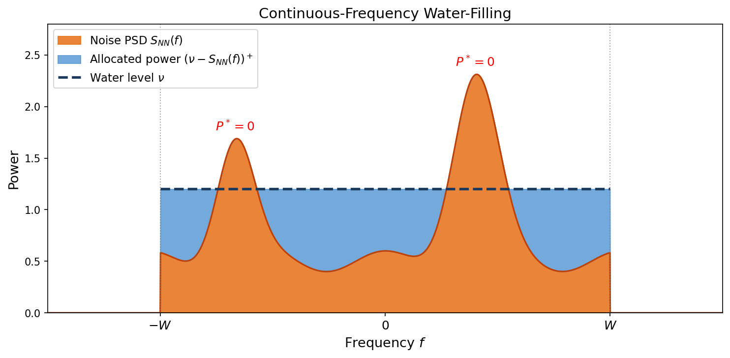
Proof idea. Decompose the channel into $n$ parallel sub-channels via the eigenvectors of the noise covariance (Toeplitz) matrix. Apply the discrete water-filling theorem (see 23.3). Take $n \to \infty$ and use Szegő’s theorem to replace the sum over eigenvalues with an integral over the PSD in normalized frequency $\hat f \in [-\frac{1}{2}, \frac{1}{2}]$. Then substitute $\hat f = {f\over 2W}$ to convert to physical frequency $f \in [-W, W]$.
23.5 Distributed Source Compression
Now we switch from channel coding to source coding. Consider a scenario where two encoders observe correlated sources and must compress them independently, i.e. without communicating with each other, then they send their independently source-coded codewords to the same decoder.
Setup: Compression and Decompression
Denote $\bold x^n := (x_1, \dots, x_n) \in \mathcal X^n$ and $\bold y^n := (y_1, \dots, y_n) \in \mathcal Y^n$ as length-$n$ sequences, as the assignments i.e. realizations of $\bold X^n$ and $\bold Y^n$, similarly defined.
- Alice observes $X_1, X_2, \dots$ and compresses by an source-coding encoder: $e_n^A : \bold x^n \mapsto w_A \in [2^{nR_A}]$.
- Bob observes $Y_1, Y_2, \dots$ and compresses by another: $e_n^B : \bold y^n \mapsto w_B \in [2^{nR_B}]$.
- $(X_k, Y_k) \sim p(x,y)$ are i.i.d. over time (for different $k$), with $x \in \mathcal X$, $y \in \mathcal Y$. In the same pair they are generally dependent on each other.
- Alice and Bob cannot communicate with each other (they encode independently).
The two rates here are defined as before.
A joint source-coding decoder receives both indices and reconstructs:
$$ d_n : [2^{nR_A}] \times [2^{nR_B}] \to \bigl((\hat X_k, \hat Y_k),\; 1 \le k \le n\bigr). $$Define the error probability (lossless reconstruction):
$$ P_e^{(n)} = \Pr\bigl(d_n(e_n^A(\bold X^n),\, e_n^B(\bold Y^n)) \ne (\bold X^n, \bold Y^n)\bigr). $$Our Question
We want to find that for which rate pairs $(R_A, R_B)$, there is a compression scheme such that the error probability approximates to zero as $n\to\infty$, i.e.
$$ \exist ((e_n^A,e_n^B,d_n),n\ge 1) \quad \text{s.t.} \lim_{n\to\infty} P_e^{(n)} = 0. $$Slepian-Wolf Theorem
Theorem (Slepian-Wolf, 1973). The rate pair $(R_A, R_B)$ is achievable (possible for communication) if and only if
$$ R_A \ge H(X \mid Y), \quad R_B \ge H(Y \mid X), \quad R_A + R_B \ge H(X, Y). $$The random binning proof below directly establishes achievability for strict inequalities ($>$). The boundary ($=$) is achieved by a closure argument: for any boundary point, take a sequence of interior points converging to it, each with a scheme satisfying $P_e^{(n)} \to 0$, so the boundary is also achievable.
The achievable region is shown below:
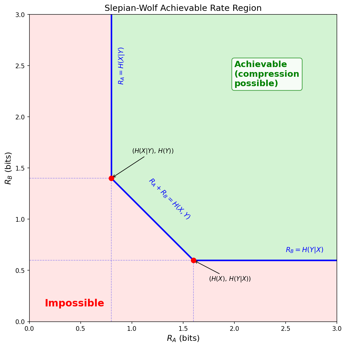
Some cases. When we are
- On the corner point $(H(X \mid Y),\, H(Y))$: Alice compresses to $H(X \mid Y)$ bits (as if Bob’s data were available as side information at the encoder). Bob compresses at the full $H(Y)$ rate.
- On the corner point is $(H(X),\, H(Y \mid X))$: the symmetric case.
- On $R_A + R_B = H(X, Y)$: the total rate equals the joint entropy, same as if the two sources were compressed jointly.
A surprising result is that independent encoding achieves the same total rate $H(X,Y)$ as joint encoding. The correlation is exploited entirely at the decoder, not at the encoders.
Proof Sketch: Random Binning
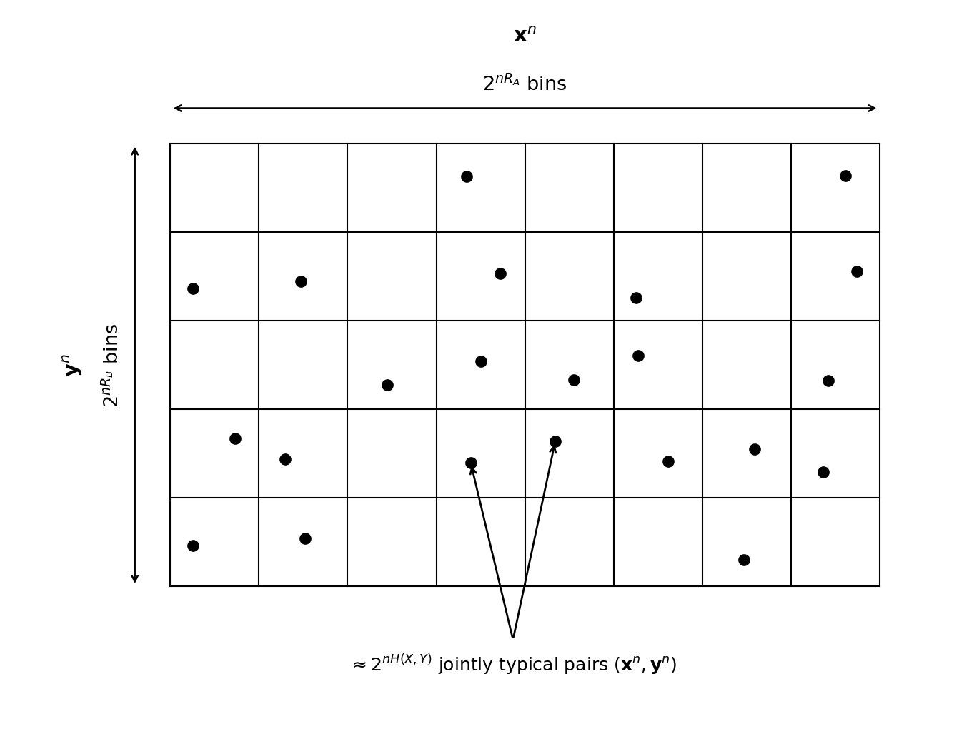
The actual encoding scheme is deterministic. The proof technique uses a random code construction to show that a good deterministic code exists: if the average error over randomly chosen codes is small, then at least one particular code must achieve that error.
The idea is random binning: distributing Alice’s $\bold x^n$ and Bob’s $\bold y^n$ into bins, which are the partitioned spaces from $\mathcal X^n \times \mathcal Y^n$.
Random code generation. Assign every $\bold x^n \in \mathcal X^n$ to one of $2^{nR_A}$ bins independently according to a uniform distribution over $[2^{nR_A}]$. Similarly, randomly assign every $\bold y^n \in \mathcal Y^n$ to one of $2^{nR_B}$ bins. Denote these random assignments $f_A$ and $f_B$. Reveal $f_A$ and $f_B$ to both the encoders and the decoder.
Encoding. Alice sends the bin index $f_A(\bold X^n)$, Bob sends $f_B(\bold Y^n)$.
Decoding. Given the received index pair $(i_0, j_0)$, the decoder declares $(\hat{\bold x}^n, \hat{\bold y}^n) = (\bold x^n, \bold y^n)$ if there is one and only one pair $(\bold x^n, \bold y^n)$ such that $f_A(\bold x^n) = i_0$, $f_B(\bold y^n) = j_0$, and $(\bold x^n, \bold y^n) \in A_{\epsilon}^{(n)}(X, Y)$. Otherwise, declare an error.
Error analysis. Here $\bold X^n$, $\bold Y^n$, $f_A$, and $f_B$ are all random. Define the error events:
$$ \begin{aligned} E_0 &= \{(\bold X^n, \bold Y^n) \notin A_\epsilon^{(n)}\}, \\ E_1 &= \{\exist \tilde{\bold x}^n \ne \bold X^n : f_A(\tilde{\bold x}^n) = f_A(\bold X^n),\; (\tilde{\bold x}^n, \bold Y^n) \in A_\epsilon^{(n)}\}, \\ E_2 &= \{\exist \tilde{\bold y}^n \ne \bold Y^n : f_B(\tilde{\bold y}^n) = f_B(\bold Y^n),\; (\bold X^n, \tilde{\bold y}^n) \in A_\epsilon^{(n)}\}, \\ E_{12} &= \{\exist (\tilde{\bold x}^n, \tilde{\bold y}^n),\, \tilde{\bold x}^n \ne \bold X^n,\, \tilde{\bold y}^n \ne \bold Y^n : f_A(\tilde{\bold x}^n) = f_A(\bold X^n),\, f_B(\tilde{\bold y}^n) = f_B(\bold Y^n),\, (\tilde{\bold x}^n, \tilde{\bold y}^n) \in A_\epsilon^{(n)}\}. \end{aligned} $$By the union bound, $P_e^{(n)} \le P(E_0) + P(E_1) + P(E_2) + P(E_{12})$.
- $P(E_0) \to 0$ by the AEP (weak law of large numbers).
- $P(E_1)$: the number of $\tilde{\bold x}^n$ jointly typical with $\bold Y^n$ is $\le 2^{n(H(X|Y)+\epsilon)}$, each falls in the same bin as $\bold X^n$ with probability $2^{-nR_A}$ (by the uniform random assignment). So $P(E_1) \le 2^{-nR_A} \cdot 2^{n(H(X|Y)+\epsilon)} \to 0$ if $R_A > H(X \mid Y)$.
- $P(E_2) \to 0$ if $R_B > H(Y \mid X)$ by symmetric argument.
- $P(E_{12}) \to 0$ if $R_A + R_B > H(X,Y)$ by the same technique.
Since the average probability of error (averaged over the random code $(f_A, f_B)$) is $< 4\epsilon$, there exists at least one deterministic code $(f_A^*, f_B^*, g^*)$ with $P_e^{(n)} < 4\epsilon$. Constructing such a code for each $n$ yields a sequence with $P_e^{(n)} \to 0$. $\square$