INFOTH Note 22: AWGN Channel and Shannon Limit
22.1 From DMC to Waveform Channels
Until now, we have met DMCs which are discrete, memoryless channels.
While the real world communication be like: a message $m$ is mapped to (corresponded to) an input waveform $x(t)$, not discrete samples.
$$ x_m(t)=\sum_{i=1}^n x_i\, g(t - iT_0), $$where $x_i$ are symbols and $T_0$ is the symbol interval.
Waveform Channel Model
$$ x(t)\to\boxed{\text{Channel}}\to y(t)=x(t)+N(t), $$- $N(t)$ is a continuous-time stochastic process (the additive noise), i.e. $(N(t), t\ge 0)$ or $(N(t), t\in \R)$.
To discuss capacity in a Shannon sense, we consider communication over a fixed time $T$. Without any constraint, the input $x(t)$ could carry infinite information (infinite amplitude, infinite bandwidth). We impose two physical constraints:
-
Power constraint (for amplitude): the transmitter has finite energy. The input waveform energy is bounded:
$$ \int_0^T |x_m(t)|^2\,dt \le \tilde P\cdot T, $$where $\tilde P$ is the allowed power (energy per unit time).
-
Bandwidth constraint: the channel (or regulations) restricts the signal spectrum to $[-W,W]$.
Consider the space of all square-integrable functions $t\mapsto x(t)$ on $[0,T]$ (i.e. $L^2([0,T])$).
By the Nyquist-Shannon sampling theorem, a signal bandlimited to $W$ in frequency is fully determined by its samples at rate $2W$, giving $2WT$ samples over duration $T$. So the bandlimited signals form a subspace of $L^2([0,T])$ with
$$ n\approx 2WT $$degrees of freedom, i.e. roughly $2WT$ orthonormal basis functions $\{\phi_i\}$ fit in this subspace, and each coefficient $x_i$ in $x(t)=\sum_i x_i\,\phi_i(t)$ can be independently chosen.
The “$\approx$” is because a signal cannot be both strictly time-limited to $[0,T]$ and strictly bandlimited to $[-W,W]$ simultaneously (uncertainty principle of Fourier Analysis). For large $WT$ the approximation is tight.
22.2 Orthogonality in Function Space
Given functions $\phi_1(t),\dots,\phi_n(t)$ in $L^2(\mathbb R)$:
Orthogonal means each has positive energy and distinct functions are uncorrelated:
$$ \int_{\mathbb R}|\phi_i(t)|^2\,dt > 0,\quad \int_{\mathbb R}\phi_i(t)\,\phi_j(t)\,dt=0,\quad i\neq j. $$Orthonormal further requires unit energy based on orthogonality:
$$ \int_{\mathbb R}\phi_i(t)\,\phi_j(t)\,dt=\begin{cases}1,&i=j,\\\\0,&i\neq j.\end{cases} $$22.3 Continuous-Time WSS Process, Autocorrelation and PSD
Continuous-Time WSS Process
A continuous-time random process $X(t)$ is wide-sense stationary (WSS) if
- its mean $E[X(t)]$ is constant over time, and
- its autocorrelation $E[X(t_1)X(t_2)]$ depends only on the time difference $\tau = t_1 - t_2$, not on the absolute times.
Autocorrelation
Under WSS, the autocorrelation function is a single-variable function:
$$ R_{XX}(\tau) = E[X(t)\,X(t+\tau)]. $$WSS simplification of autocorrelation.
For a general (non-WSS) random process $X(t)$, the autocorrelation is a function of two time instants:
$$ R_X(t_1, t_2) := E[X(t_1) X(t_2)]. $$This can depend on both $t_1$ and $t_2$ individually. Under WSS, it simplifies to a function of the lag $\tau = t_1 - t_2$ alone:
$$ R_X(t_1, t_2) = R_X(t_1 - t_2). $$Some basic properties of the WSS autocorrelation:
- $R_X(0) = E[X(t)^2]$ is the average power of the process.
- $|R_{XX}(\tau)| \le R_X(0)$ (by Cauchy-Schwarz).
- $R_X(-\tau) = R_{XX}(\tau)$ (symmetry).
Power Spectral Density
The power spectral density (PSD) is the Fourier transform of the autocorrelation function, of frequency $f$:
$$ S_{XX}(f) = \int_{\mathbb R} R_{XX}(\tau)\,e^{-j2\pi f\tau}\,d\tau. $$$S_{XX}(f)$ describes how the power of $X(t)$ is distributed across different frequencies.
For a bandlimited process (e.g. the waveform channel here, supported on $[-W, W]$), $S_{XX}(f) = 0$ outside $[-W, W]$, and the total power is $\int_{-W}^{W} S_{XX}(f)\,df$.
A process whose PSD is constant (flat) across all frequencies is called white. If the noise power varies with frequency (i.e. the noise is colored), the optimal power allocation across frequencies follows the water-filling strategy (see Note 23).
We actually pay attention to the noise power not the input or output, i.e. $S_{NN}(f)$ and $R_{NN}(\tau)$, while $X$ above is purely a notation.
22.4 White Gaussian Noise
Definition
- $N(t)$ is a Gaussian process: for any finite set of times $t_1,\dots,t_k$, the vector $(N(t_1),\dots,N(t_k))$ is jointly Gaussian.
- It is white: its PSD is $S_{NN}(f):={N_0\over 2}$, a constant across all frequencies (“white” = flat spectrum). Equivalently, the autocorrelation is $R_{NN}(\tau)=\frac{N_0}{2}\delta(\tau)$, so $N(t_1)$ and $N(t_2)$ are uncorrelated (and hence independent, by Gaussianity) whenever $t_1\neq t_2$.
We say white Gaussian noise is WSS because it satisfies the WSS condition (See 23.4), and after that we say a constant PSD under this case is called white.
The total noise power in a band $[-W,W]$ is then
$$ \int_{-W}^{W}\frac{N_0}{2}\,df = N_0\,W. $$So $N_0$ itself is the noise power per unit one-sided bandwidth, which is a cleaner quantity.
Property
Given an orthonormal basis $\{\phi_i\}$, define the projection coefficients (the components in orthogonal directions) of $N(t)$ onto the basis:
$$ N_i := \int_{\mathbb R} N(t)\,\phi_i(t)\,dt. $$Then $N_1,\dots,N_n$ are i.i.d. $\mathcal N(0,\,{N_0\over 2})$. This follows from: Gaussian (projections of a Gaussian process are Gaussian) + white (flat PSD means each direction gets equal variance ${N_0\OVER 2}$, and orthogonal projections are uncorrelated, hence independent by Gaussianity).
Why i.i.d. with Variance ${N_0\over 2}$?
More explicitly, the variance of each projection is $$ \mathrm{Var}(N_i) = \int_{\mathbb R} S_{NN}(f)\,|\Phi_i(f)|^2\,df = \frac{N_0}{2}\int_{\mathbb R}|\Phi_i(f)|^2\,df = \frac{N_0}{2}, $$where the last step uses Parseval’s theorem ($\|\Phi_i\|^2 = \|\phi_i\|^2 = 1$ by orthonormality).
The reason why we project onto an orthonormal basis is that the noise $N(t)$ is a continuous-time object with uncountably many random values. Projecting onto $\{\phi_i\}$ decomposes it into finitely many i.i.d. scalar Gaussian random variables, reducing the problem to standard probability. This is what leads to the AWGN model.
22.5 AWGN: Additive White Gaussian Noise
- Input alphabet $=\mathbb R$.
- Output alphabet $=\mathbb R$.
- Channel model: $Y\mid X=x \sim \mathcal N(x,\sigma^2)$.
We want the channel capacity $C$ in this continuous-time setting, i.e. the largest rate $R$ (bits per channel use) at which we can communicate with error probability to zero, as block length $n\to\infty$.
Simplification
The full waveform channel $x(t)\to y(t)$ is a continuous-time problem. After projecting onto an orthonormal basis $\{\phi_i\}$, it decomposes into $n$ independent scalar AWGN channels $Y_i = x_i + N_i$. Each scalar channel is one “channel use” (one degree of freedom, not one time step). We first study this single scalar channel $Y=X+N$, then combine $n$ uses in 22.7.
完整的波形信道 $x(t)\to y(t)$ 是连续时间问题。投影到 orthonormal basis $\{\phi_i\}$ 后,分解为 $n$ 个独立的标量 AWGN 信道 $Y_i = x_i + N_i$。每个标量信道就是一次"信道使用"(一个自由度,不是一个时间点)。我们先研究单个标量信道 $Y=X+N$,再在 22.7 中组合 $n$ 次使用。
The connection between $\sigma^2$ and ${N_0\OVER 2}$, and between the per-use power $P$ and the waveform power $\tilde P$, is also made in 22.7.
Encoding and Decoding
Composition and Decomposition from Coefficients
Each $x_i(m)$ is a scalar (coefficient) chosen by the encoder as input to the $i$-th AWGN channel use.
The encoder constructs from the message $m$ deterministically using the orthonormal basis:
$$ x_m(t)=\sum_{i=1}^n x_i(m)\,\phi_i(t). $$At the receiver, projecting $x(t)+N(t)=y(t)$ onto $\{\phi_i\}$ gives $Y_i = x_i(m) + N_i$ independently for each $i$.
Block Coding and Power Constraint
The waveform $x(t)$ has $n$ degrees of freedom (from 22.1), in other words, is a weighted sum of $n$ orthonormal functions $\{\phi_i\}$, where in the bandwidth constraint $n\approx 2WT$.
So projecting onto an $n$-dimensional orthonormal basis $\{\phi_i\}$ reduces it to a codeword (or a vector/block) in $\mathbb R^n$.
Each group of a function $\phi_i$ with the coefficient $x_i(m)$ and the random variables $Y_i$ and $N_i$ is defined within the $i$-th channel use, and the block length $n$ is the number of channel uses (one per basis function).
There are $M_n = 2^{nR}$ messages. Each message $m$ can be viewed as an $nR$-bit string (its binary index). The encoder maps each message to a codeword of length $n$:
$$ e_n:[M_n]\to\mathbb R^n,\quad e_n:m\mapsto (x_1(m),\dots,x_n(m)),\quad M_n=2^{nR}, $$subject to the per-codeword power constraint:
$$ \frac{1}{n}\sum_{i=1}^n x_i^2(m)\le P,\quad \forall\, m\in[M_n]. $$Here $P$ is the allowed energy per channel use.
The decoding map takes the received vector $Y^n=(Y_1,\dots,Y_n)\in\mathbb R^n$ and outputs a message index or declares give-up by the asterisk:
$$ d_n:\mathbb R^n\to [M_n]\cup\{*\}. $$Error Probabilities
Same definitions as the DMC case (see Note 18):
- Conditional error probability for message $m$:
- Maximal error probability:
- Average error probability:
22.6 AWGN Shannon Theorem
Achievability and Converse Theorem
The form is like the DMC case. The bound is different though. The capacity is
$$ C = \frac{1}{2}\log\!\left(1 + \frac{P}{\sigma^2}\right) \text{ bits per channel use}, $$so we have
- Achievability: If $R\lt C$ bits per channel use, then $\exists\,((e_n,d_n),\,n\ge 1)$ s.t. $|M_n|=2^{nR}$ and $\lambda_{\max}^{(n)}\to 0$.
- Converse: If $R>C$, then $\forall\,((e_n,d_n),\,n\ge 1)$, $\liminf_n P_e^{(n)}>0$.
- Bits per channel use for this channel-use case. We want a bits-per-unit-time form later in 22.7.
Proof Sketch
We have only proved the Shannon theorem for DMC, not for AWGN. Below is the intuitive proof sketch behind the formula.
Recall: Weakly Typical Set
Given $X_1,X_2,\dots$ i.i.d. $\mathbb R$-valued with density $f(x)$ having differential entropy $h(X)$, the weakly typical set is
$$ A_\epsilon^{(n)}=\bigg\{(x_1,\dots,x_n)\in\mathbb R^n:\bigg|-\frac{1}{n}\log\prod_{i=1}^n f(x_i)-h(X)\bigg|\le\epsilon\bigg\}. $$We have the intuition
$$ 2^{n(h(X)-\epsilon)}\le \operatorname{Vol}(A_\epsilon^{(n)})\le 2^{n(h(X)+\epsilon)}. $$Mutual Information Maximization
$\frac{1}{2}\log(1+P/\sigma^2)$ is the solution to
$$ \max_{f_X}I(X;Y)=\max_{f_X}\big[h(Y)-h(Y|X)\big], $$subject to $E[X^2]\le P$, where $Y=X+N$, $N\sim\mathcal N(0,\sigma^2)$, $X\perp\!\!\!\perp N$.
Since $h(Y|X)=h(N)=\frac{1}{2}\log(2\pi e\,\sigma^2)$, we want to maximize $h(Y)$ subject to $E[Y^2]\le P+\sigma^2$.
The Gaussian $Y\sim\mathcal N(0,P+\sigma^2)$ would be best if possible (and it is, by choosing $X\sim\mathcal N(0,P)$). This gives
$$ C = \frac{1}{2}\log(2\pi e(P+\sigma^2)) - \frac{1}{2}\log(2\pi e\,\sigma^2)= \frac{1}{2}\log\!\left(1+\frac{P}{\sigma^2}\right). $$Volume Intuition
$$ \operatorname{Vol}(A_{\epsilon,Y}^{(n)})\approx 2^{n\cdot\frac{1}{2}\log 2\pi e(P+\sigma^2)},\qquad \operatorname{Vol}(A_{\epsilon,N}^{(n)})\approx 2^{n\cdot\frac{1}{2}\log 2\pi e\,\sigma^2}. $$The ratio of these two volumes is
$$ \frac{\operatorname{Vol}(A_{\epsilon,Y}^{(n)})}{\operatorname{Vol}(A_{\epsilon,N}^{(n)})}\approx 2^{n\cdot\frac{1}{2}\log(1+P/\sigma^2)}. $$22.7 From Scalar AWGN to Waveform Capacity
We now connect the scalar AWGN capacity (22.6) with the waveform channel parameters from 22.1.
Setup
- Bandwidth $W$ (freq.), communication duration $T$ (time).
- Waveform power constraint $\tilde P$ (energy per unit time), so total energy $= \tilde P \cdot T$.
- Number of degrees of freedom (orthonormal basis functions): $n \approx 2WT$.
From here on we assume $n = 2WT$ (not $n\approx 2WT$), since the capacity formula is an asymptotic result ($n\to\infty$), and the error from approximity becomes negligible.
Identifying parameters:
-
Noise variance. Each $N_i \sim \mathcal N(0, {N_0\OVER 2})$ (from 22.4), so the scalar AWGN channel has $\sigma^2 = {N_0\OVER 2}$.
-
Per-use power. The total energy $\tilde P \cdot T$ is shared equally among $n = 2WT$ channel uses, so the energy per use is:
Derivation of Waveform Capacity
Each of the independent $n = 2WT$ scalar channels has capacity $\frac{1}{2}\log(1 + P/\sigma^2)$ bits (from 22.6).
Over time $T$, the total number of reliably transmittable bits is at most:
$$ n \cdot \frac{1}{2}\log\!\left(1+\frac{P}{\sigma^2}\right) = \frac{2WT}{2}\log\!\left(1+\frac{\tilde P/2W}{{N_0\OVER 2}}\right) = WT\log\!\left(1+\frac{\tilde P}{N_0 W}\right) \text{ bits}. $$Dividing by $T$ gives the capacity per unit time:
$$ \boxed{\tilde C = W\log \left(1+\frac{\tilde P}{N_0 W}\right)\quad\text{bits per unit time}.} $$- $W$: bandwidth (frequency), $\tilde P$: power (energy/unit time), $N_0$: noise spectral density;
- $\tilde P\over N_0 W$: Signal-Noise Ratio (SNR) within the band with bandwidth $W$.
- Convention:
- $C = \frac{1}{2}\log(1+P/\sigma^2)$ is bits per channel use (22.6); the rate in DMC is bits per channel use;
- $\tilde C = W\log(1+\tilde P/(N_0 W))$ is bits per unit time. Same tilde convention as $R$ vs. $\tilde R$ and $P$ vs. $\tilde P$.
22.8 Spectral Efficiency & Shannon Limit
Bit Rate
The bit rate is sent bits per unit time:
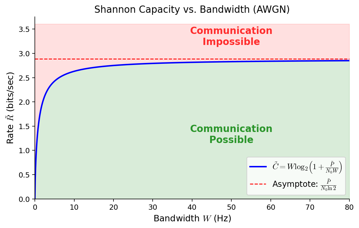
$$ \tilde R = {nR\over T}. $$Reliable communication requires $\tilde R < \tilde C = W\log \left(1+\frac{\tilde P}{N_0 W}\right)$ as above.
横轴为 $W$,纵轴为 $\tilde R$。在 $\tilde C = W\log_2(1+\tilde P/(N_0 W))$ 以下,则可以进行通信。当 $W\to\infty$ 时,$\tilde C\to \tilde P/(N_0\ln 2)$(渐近线)。
Spectral Efficiency
$$ \mathfrak{R}={\tilde R\over W} $$In SI unit, the unit is bits/sec/Hz or bits solely.
Signal-to-Noise Ratio per Bit (Ebno)
Define the energy per bit:
$$ E_b := \frac{\tilde P}{\tilde R}, $$i.e. transmit power divided by bit rate (energy per bit). $E_b/N_0$ is called the signal-to-noise ratio per bit (or Ebno), and is dimensionless (both $E_b$ and $N_0$ have the same dimension: energy).
The SNR within the band is:
$$ \text{SNR} = \frac{\tilde P}{N_0 W} = \frac{E_b\,\tilde R}{N_0\,W} = \frac{E_b}{N_0}\cdot\mathfrak{R}. $$Substituting into $\tilde R < \tilde C$, i.e. $\mathfrak{R} < \log_2(1+\text{SNR})$:
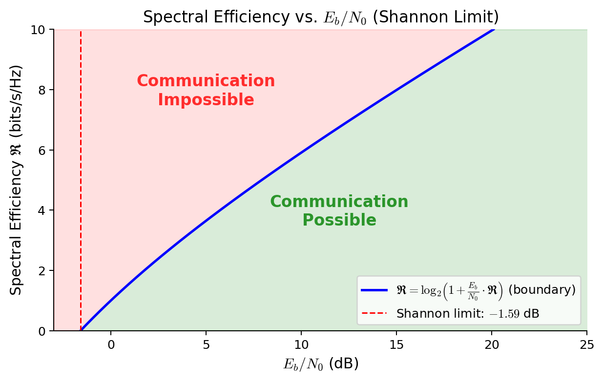
$$ \mathfrak{R} < \log_2\!\left(1+\frac{E_b}{N_0}\cdot\mathfrak{R}\right). $$Lower Bound of Ebno
Rearranging the inequality above:
$$ \frac{E_b}{N_0}>\frac{2^{\mathfrak R}-1}{\mathfrak R}=:f(\mathfrak R). $$The function $f(\mathfrak R)$ is strictly increasing on $(0,\infty)$: its derivative’s numerator is $g(\mathfrak R)=\mathfrak R\cdot 2^{\mathfrak R}\ln 2 - 2^{\mathfrak R}+1$, which satisfies $g(0)=0$ and $g'(\mathfrak R)=\mathfrak R\cdot 2^{\mathfrak R}(\ln 2)^2>0$, so $g>0$ for $\mathfrak R>0$. Therefore the infimum of $f$ is attained as $\mathfrak R\to 0^+$:
$$ \inf_{\mathfrak R>0}f(\mathfrak R)=\lim_{\mathfrak R\to 0^+}\frac{2^{\mathfrak R}-1}{\mathfrak R}=\ln 2\approx 0.693. $$So for any $\mathfrak R > 0$:
$$ \frac{E_b}{N_0}>\ln 2, $$or in decibels:
$$ \left(\frac{E_b}{N_0}\right)_{\min} = 10\log_{10}(\ln 2)\approx -1.59\text{ dB}. $$This is the Shannon limit: the absolute minimum $E_b/N_0$ for reliable communication over an AWGN channel, regardless of bandwidth, spectral efficiency, or coding scheme.