INFOTH Note 18: Channel Coding Theorem for DMC 1

18.1 Communication

Setup

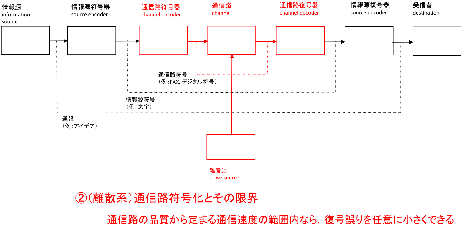
There is a sender and a receiver in a communication.

• A sender has a message \(m\in[M]:=\{1,2,\dots,M\}\) to send

  • The information source codeword (情報源符号): \(m\), inputted into a channel encoder, encoded into \(x\in\mathcal X\)
  • Approximately a channel encoder

• The sender sends a message via a channel. The channel is noisy, mapping \(x\) to \(y\) probably:

  \[ x\to\underbrace{\boxed{p(y|x)}}_W\to y \]

• A receiver receives \(y\) and wants to decode \(y\) into the original message \(m\), but turning out to be \(\hat m\):

  • The channel outputs \(y\) and the receiver uses a channel decoder to recover \(\hat m\simeq m\)
  • Approximately a channel decoder

18.2 Discrete Memoryless Channel Model

In this channel, we have \(x\in\mathcal X\) and \(y\in\mathcal Y\) where \(\mathcal X\) is the input alphabet and \(\mathcal Y\) is the output alphabet.

The channel probability modeling is \(p(y|x),x\in\mathcal X,y\in\cal Y\).

The “transition” probability in this channel satisfies \(p(y|x)\ge 0,\sum_y p(y|x)=1,\forall x\in\mathcal X\).

Sender: Channel Encoder

Given we have \(n\) uses for this channel (the sent thing is \(x_1x_2\dots x_n\)), i.e. the sender’s codeword is a \(n\)-length sequence, the encoder is a map:

where we have \(M_n\) messages.

Receiver: Channel Decoder

The decoder is a map:

where we recover the message and we can also give up by the asterisk.

Memoryless Assumption (Property)

We say the channel is memoryless by

i.e.

We get

Conditional Probabilities of Error

We define the probability of error given \(i\) is the message:

and the max probability of error:

and the average probability of error:

here we has a prior that every message shares equal probability of \(\frac1 {M_n}\) though in reality it can follow any \(p(x)\).

Goal

We want to minimize the probability of error to zero.

Def: Rate

If we have a real-valued rate, \(M_n\) can be \(\lceil 2^{nR}\rceil\).

Some Properties

• We are choosing a subset of \(\mathcal X^n\) for the image of \(e_n\), say \(\mathcal C\subseteq \mathcal X^n\). We can define \(\mathcal C=\{\bold x^n(1),\bold x^n(2),\dots,\bold x^n(m)\}\).
• If \(\mathcal C=\mathcal X^n\), i.e. \(M_n=|\mathcal X^n|=n|\mathcal X|\), then \(R=R_{\max}=\log|\mathcal X|\) and every sequence in \(\mathcal X^n\) is used, thus we cannot detect errors nor correct them. So for an error-detectable and correctable code, \(R<R_{\max}=\log|\mathcal X|\).
• \(\eta={R\over R_{\max}}\) is called the efficiency 効率/code rate 符号化率 of \(\mathcal C\). The redundancy 冗長度 is \(\rho=1-\eta\).

18.3 Shannon’s Channel Coding Theorem for DMC

Setup: Capacity

Define the ==capacity== of a channel (DMC):

where \(Y|(X=x)\sim (p(y|x),\forall y\in\mathcal Y)\).

Given the conditional probability fixed, the mutual information is concave over \(p(y)\) and \(p(x)\) so we can find a maximum value for the capacity.

We can also compute the capacity like this:

where the blue ones are unknown/not fixed.

Since the MI is the difference between entropies,

Generally, the computing procedures can be:

1. Given the transition probability matrix \(P\), every row is for a \(x\) and every column is for a \(y\);
2. Compute the conditional entropy \(H(Y|X)\).
3. Compute the output entropy \(H(Y)\).
4. Plug them into the MI and find the max.

Symmetric Capacity

(From Note 21) When \(X\) follows a uniform distribution: \(p(x)=\frac1{|\mathcal X|}\), we define

For a BISO channel with binary input, the uniform input gives \(H(X)=1\), so

Theorem

For any \(R<C\), there exists a collection of pairs of encoder-decoders \(((e_n,d_n),n\ge 1)\) s.t.

Note here \(M_n=\lceil 2^{nR}\rceil\) must be the message alphabet size for every \(n\) and the fixed \(R\).

Another Proposition

For any \(R>C\), every collection of pairs of encoder-decoders will make the error probability larger than 0.

No strategy exists making the error prob. approaching 0.

Def: Jointly Weakly Typical Set

Define \(A_{\epsilon,X,Y}^{(n)}\subseteq \mathcal X^n\times \mathcal Y^n\) s.t.

where

Then we have some bounds.

and for the cardinality,

Proof Sketch (“Probabilistic Method”)

Proof Sketch.

Suppose the input sequence to the channel \(X_1,\dots,X_n\) are i.i.d. \((p(x),x\in\mathcal X)\).

Then outputs will also be i.i.d. \((p(y),y\in\mathcal Y)\) where \(p(y):=\sum_x p(x)p(y|x)\).

Roughly \(2^{nH(Y)\pm n\epsilon}\) output sequences occupy all the probabilities in \(\mathcal Y^n\) (roughly they are weakly typical).

For each weakly typical input sequence \(\bold x^n\) roughly \(2^{n H(Y|X)\pm n\epsilon}\) output sequences \(\bold y^n\) occupy all the probabilities conditioned on \(\bold x^n\).

So there exists a “ball” as the weakly typical subset of \(\mathcal Y^n\), with about \(2^{nH(y)\pm n\epsilon}\) output sequences. And there are many small subsets with \(2^{nH(Y|X)\pm n\epsilon}\) output sequences filling the ball, each corresponding to only 1 \(\bold x^n\) instance.

Review this statement. We have small balls, each related to only 1 input sequence, with about \(2^{nH(Y|X)\pm n\epsilon}\) output sequences in the ball. They fill up the whole typical set for \(\bold y^n\). So we can recover \(\bold x^n\)’s from typical \(\bold y^n\)’s. But if we have untypical ones, we give up by recovering an asterisk.

18.4 Examples of DMCs w/ Capacities

Binary Symmetric Channel (BSC)

graph LR
    subgraph X
        x0("0")
        x1("1")
    end
    subgraph Y
        y0("0")
        y1("1")
    end
    x0 -- "1-a" ----> y0
    x0 -- "a" --> y1
    x1 -- "a" --> y0
    x1 -- "1-a" --> y1

• The setup of \(\text{BSC}(a)\): \(\mathcal X=\mathcal Y=\{0,1\}\), \(p(y|x)\) follows \(p(1|1)=p(0|0)=1-a\), \(p(0|1)=p(1|0)=a\). \(a\in[0,1]\).
• We can assume \(0\le a\le \frac12\) as well since if \(a>\frac12\) the symbol 0/1 can be exchanged.
• \(p(x)\) is unknown here, still.

We denote the binary Shannon entropy as \(h(\cdot)\), and

where \(H(Y)\) can be 1 when \(p(y)=(\frac12,\frac12)\) and thus \(p(x)\) is also decided as \((\frac12,\frac12)\).

• if \(a=0\), then the capacity is 1 (a noiseless channel)
• if \(a=\frac12\), the capacity is 0, so no rate can have a good way.

Binary Erasure Channel (BEC)

graph LR
    subgraph X
        x0("0")
        x1("1")
    end
    subgraph Y
        y0("0")
        y1("1")
        ye("e")
    end
    x0 -- "1-b" ----> y0
    x0 -- "b" --> ye
    x1 -- "b" --> ye
    x1 -- "1-b" --> y1

• Every input may be erased by \(a\) probability
• Setup: \(\mathcal X=\{0,1\}\), \(\mathcal Y=\{0,1,e\}\), \(p(y|x)=b,\forall y\ne x\), otherwise \(p(y|x)=1-b\).

Let \(p_X(0)=u\).

We see

Hence

so

where the maximum holds at \(u=\frac12\) i.e. \(p(x)=(\frac12,\frac12)\) and \(p_Y(0)=p_Y(1)=\frac12(1-b)\) and \(p_Y(e)=b\).

Binary Input Symmetric Output (BISO)

Def: Involution Map

A map \(\pi:\mathcal Y\to\mathcal Y\) is called an involution iff \(\pi\circ \pi=\mathbf I\) (identity map) i.e. \(\pi^{-1}=\pi\).

Def: BISO Channel

A channel is a BISO channel iff the input alphabet is \(\mathcal X=\{0,1\}\) and in the transition probability \(P\), \(P_{y,0}=P_{\pi(y),1}\) holds for every \(y\in\mathcal Y\) where \(\pi\) exists as an involution, i.e.

BSC is a special example of BISO, where \(\pi(0)=1,\pi(1)=0\).

BEC is a special example of BISO, where \(\pi(0)=1,\pi(1)=0,\pi(e)=e\).

Symmetric Channels

The channels where for the transition probability matrix,

• every row is the permutation of each other row \(\implies H(Y|X=x)\) is the same, \(\forall x\)
• every column is the perm. of each other col. \(\implies \sum_x p(y|x)=c\), a constant, \(\forall y\)

Examples: 1) \(P=\begin{bmatrix}0.3&0.2&0.5\\0.5&0.3&0.2\\0.2&0.5&0.3\end{bmatrix}\); 2) \(Y=(X+Z)\mod c\).

For these channels, let \(\bold r\) be any row of \(P\), \(H(Y|X)=H(\bold r)\) since \(H(Y|X=x)\) keeps the same regardless of what \(x\) is, then we have

with equality if \(p(y)\) is uniform since we won’t consider \(H(Y|X)\) anymore.

Here a uniform \(p(x)=\frac1{|\mathcal X|}\) can achieve a uniform distribution on \(Y\):

Weakly Symmetric Channels

The channels where for the transition probability matrix,

• every row is the permutation of each other,
• every column sums up to the same value (looser than symmetric channels)

Examples: \(P=\begin{bmatrix}1/3&1/6&1/2\\1/3&1/2&1/6\end{bmatrix}\) is weakly symmetric but not symmetric.

The capacity and the uniform achievement is still the same:

achieved by a uniform distribution on the input alphabet \(p(x)=\frac1{|\mathcal X|}\).