[Flow] Rectified Flow Explained
Reading Flow Matching Across Domains Vol. 1
Here is the (simple) explanation for the framework Rectified Flow.
Overview
Rectified Flow (RF) is a generative modeling method, which tries to transport data from source distribution \(\pi_0\) (which corresponds to the pure Gaussian distribution \(\pi_0=N(0,I)\)) and the target distribution \(\pi_1\), which is the distribution of clean images.
The overall objective is to align the velocity estimate (using the UNet, denoted as \(v_\theta\) now) to the actual velocity between the source image \(X_0\) and the target image \(X_1\). First, the timesteps here are all normalized between \(t\in[0,1]\), instead of spreading in \(\{0,\cdots, T\}\).
For a general case when \(t\in[0,T']\), the velocity is \(X_1-X_0\over T'\) while the displacement is \(X_1-X_0\). Upon being normalized i.e. \(T'=1\), we can numerically equal these two quantities.
We define the interpolation path as
\[ X_t=tX_1+(1-t)X_0,\qquad t\in[0,1]\tag{1} \]where \(X_0\sim \pi_0,X_1\sim\pi_1\). Then, the time-conditional objective is
\[ \min_\theta \int_0^1 \mathbb{E} \left[ \| (X_1 - X_0) - v_\theta(X_t, t) \|^2 \right] \mathrm d t\tag{2.1} \]where we can see the objective (loss) is weighted equally over \(t\in[0,1]\), equivalent to another expectation operator over a uniform distribution over the continuous time \(t\).
Adding the class conditioning where \(X_1\sim \pi_1|c\):
\[ \min_\theta \int_0^1 \mathbb{E} \left[ \| (X_1 - X_0) - v_\theta(X_t, t, c) \|^2 \right] \mathrm d t.\tag{2.2} \]From the core of objective we can see, we want the path as straight (as a hyperline from \(X_0\) to \(X_1\)) as possible, i.e. rectified flow requires a fixed velocity from \(X_0\) to \(X_1\); though it will be curved as not ideal.
Since we don’t know target \(X_1\) in generation, and even \(X_0\) is not an input into \(v_\theta\), in some position (\(t\), \(X_t=x\)) many \(X_0,X_1\) hyperlines will intersect, so an optimal estimate \(v^*(t, X_t)\) will be (realized as)
\[ v^*(t,x)=\mathbb E[X_1-X_0|X_t=x]\tag{2.3} \]as a max likelihood estimate (MLE) form, \(v^*(t,x,c)=\mathbb E[X_1-X_0|X_t=x,c]\) when conditioned.
Training
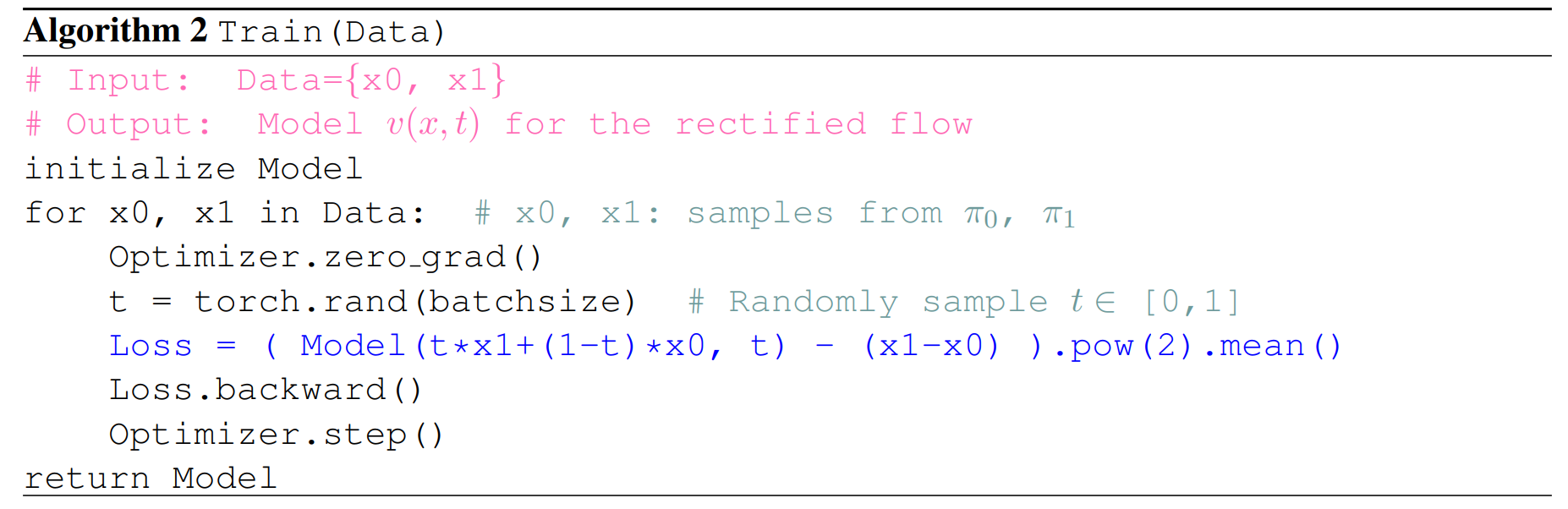
For an RF, the objective is listed above, which is to minimize uniformly over the whole dataset and also over all times \(t\).
However, as we all know we can only estimate the integral \(\int_0^1\) and the integral behind the \(\mathbb E\) symbol, instead of directly computing.
For a time-conditional RF, using the Monte Carlo integral method, we can estimate the objective (loss) by
\[ L=\int_0^1 \mathbb{E} \left[ \| (X_1 - X_0) - v_\theta(X_t, t) \|^2 \right] \mathrm d t \approx\frac1n\sum_{i=1}^n ||x_{1}^{(i)}-x_0^{(i)}-v_\theta(x_t^{(i)},t^{(i)})||^2\tag{3.1} \]where \(x_1^{(i)}\) is a data point (a clean image) drawn from the target distribution \(\pi_1\) (the training dataset), \(x_0^{(i)}\) is drawn from the source distribution \(\pi_0\), conventionally a dynamically-generated Gaussian noise (if we want a generator from the standard normal distribution), and \(x_t^{(i)}\) is the interpolation where the timestep \(t^{(i)}\) is sampled from a distribution of timesteps. The distribution of \(t\) can be (most naturally) a continuous uniform, a discrete uniform on \(\{0,\cdots, T\}\) (discretized continuous schedule) or other nonlinear schedules such as sigmoid(1-d Gaussian r.v.).
For a class-conditional RF (while time condition is still existing), the estimate is
\[ L=\int_0^1 \mathbb{E} \left[ \| (X_1 - X_0) - v_\theta(X_t, t, c) \|^2 \right] \mathrm d t \approx\frac1n\sum_{i=1}^n ||x_{1}^{(i)}-x_0^{(i)}-v_\theta(x_t^{(i)},t^{(i)},c^{(i)})||^2\tag{3.2} \]where the expectation is over time \(t\), condition \(c\), \(X_1\sim \pi_1|c\) and \(X_0\sim \pi_0\) as usual; \(c^{(i)}\) is the class paired with the drawn \(x_1^{(i)}\).
The loss can be regarded as a L2 loss between the predicted velocity and the real displacement too. The algorithm is shown below:
Sampling
For a RF, we build an ODE to sample. The ODE setup for a time-conditional RF is
\[ \frac{dZ_t}{dt} = v_\theta(Z_t, t), \quad Z_0 \sim \pi_0\tag{4.1} \]and we want \(Z_1\) as the generated image. The general form of the solution is
\[ Z_t = Z_0 + \int_{0}^{t} v_\theta(Z_s, s)\mathrm ds.\tag{5.1} \]Similarly, this integral is also not directly computable. We can use ODE solver (solving methods) to estimate this as well.
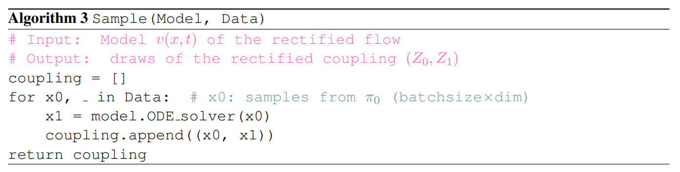
The methods can be Euler’s method or RK45, and we implement the former in the repo as a simple but working one.
The estimate for \(Z_1\), using Euler’s method, is
\[ Z_1\approx Z_0+{1\over T}\sum_{k=0}^{T-1}v_\theta(Z_{k/ T},{k\over T})\tag{6.1} \]where \(\frac1T\) works as the sampling step size \(\Delta t\). A RF trained with a discrete-uniform-scheduled time can naturally match the stepping and a same step size.
For a class-conditional RF, the framework is similar, but we specify the class \(c\), so we have
\[ \frac{dZ_t}{dt} = v_\theta(Z_t, t,c), \quad Z_0 \sim \pi_0\tag{4.2}, \]\[ Z_t = Z_0 + \int_{0}^{t} v_\theta(Z_s,s, c)\mathrm ds,\tag{5.2} \]and the estimate
\[ Z_1\approx Z_0+{1\over T}\sum_{k=0}^{T-1}v_\theta(Z_{k/ T},{k\over T},c)\tag{6.2}. \]Implementation Detail and Results
I implemented two kinds of RF (time/class-conditional) based on the structure of DDPM.
I used the time-conditional UNet for the time-conditional RF, and the class-conditional UNet for the class-conditional one. The architecture of this core model remains same as in DDPM.
Beta schedules (the list) is no longer needed, but the number of timesteps as a hyperparameter is still necessary for the forward and sampling methods to generate an estimate.
For the class-conditional RF, the Classifier-free Guidance (CFG) is also slightly changed to guide the conditioned velocity estimate instead of the noise estimate, from the unconditioned counterpart:
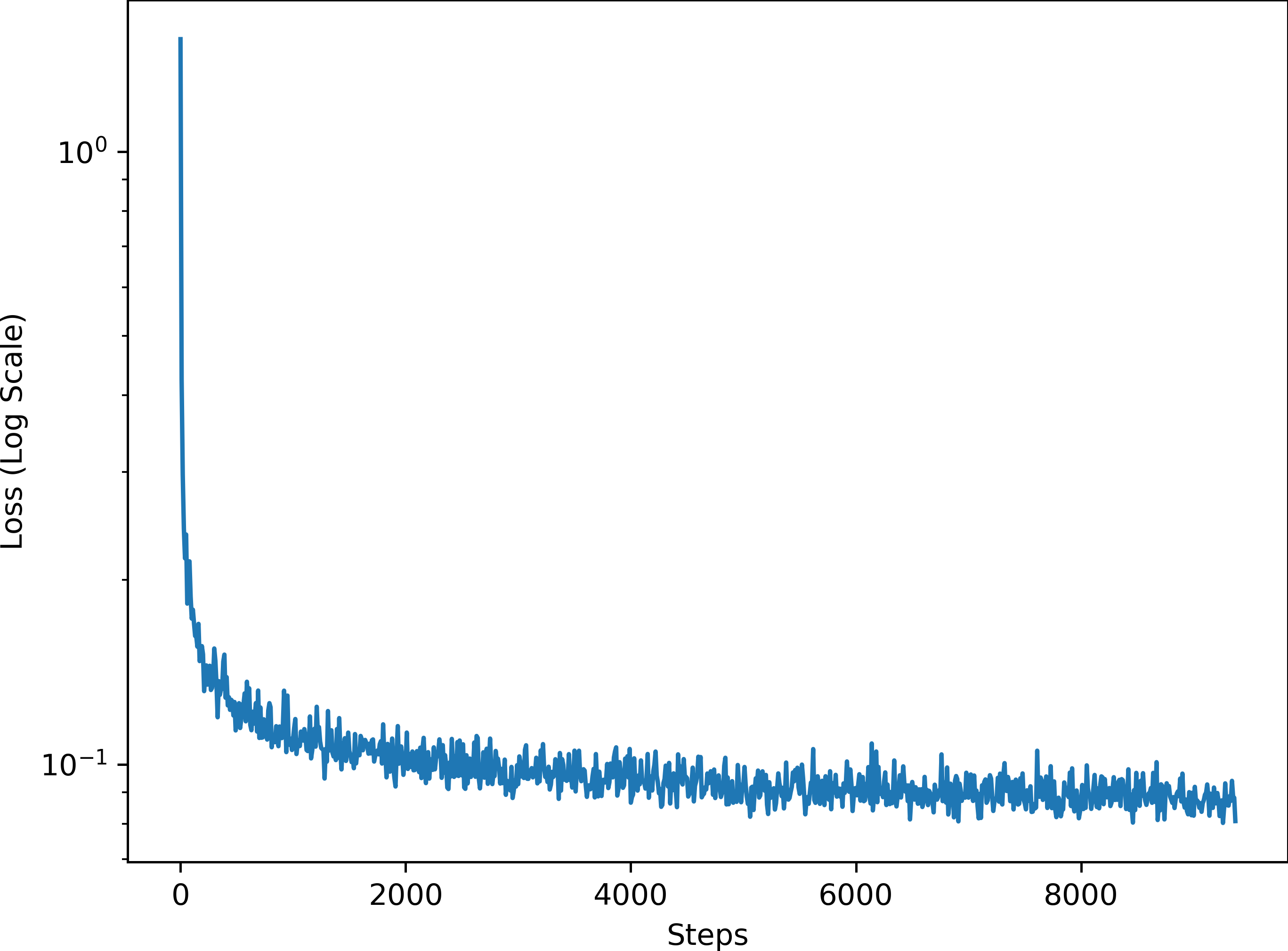
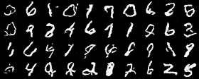
\[ Z_1\approx Z_0+{1\over T}\sum_{k=0}^{T-1}\gamma v_\theta(Z_{k/ T},{k\over T},c)+(1-\gamma)v_\theta(Z_{k/ T},{k\over T},0) \tag{7}. \]We train with the same set of hyperparameters as in 2.2. The training and testing loss are higher than those in DDPM training, but the generated (sampled) images are fairly good and unnoised.
Results of Time-Conditional RF
The training loss curve for the time-conditional RF is shown below.
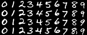
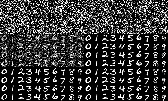
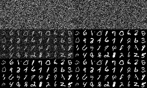
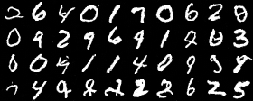
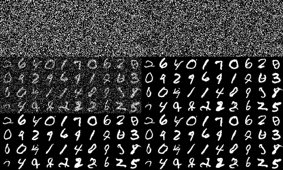
The sampling results for the time-conditional RF are shown below.
Results of Class-Conditional RF
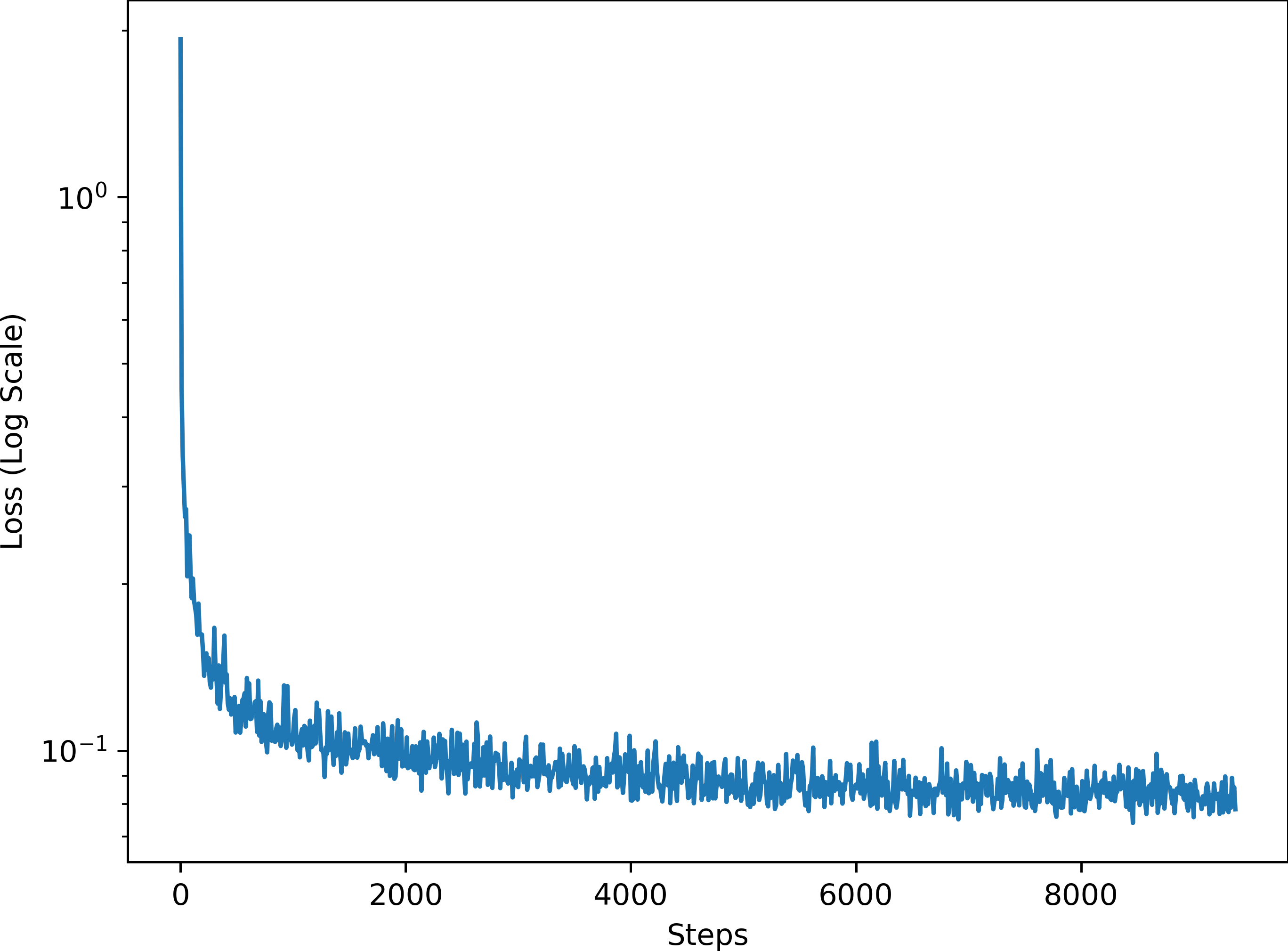
The training loss curve for the class-conditional RF is shown below.
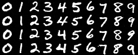
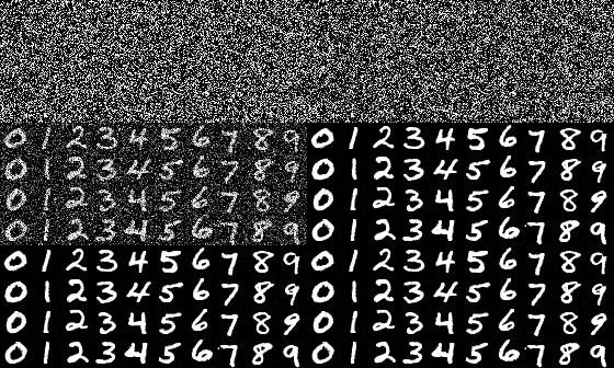
The sampling results for the class-conditional RF are shown below.