Programming Project #2 (proj2)
COMPSCI 180 Intro to Computer Vision and Computational Photography
Chuyan Zhou
This webpage uses the Typora Newsprint theme of markdown files.
Part 1: Fun with Filters
1.1 Finite Difference Operator
Here we have the finite difference operators respectively horizontal and vertical as
To compute the gradient which is given by
where
and we have the right as the original point for scipy.signal.convolve2d where the mode is 'same' (the size of the result is kept same as the original image
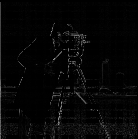
To find the magnitude from the gradients, we use
written as elementwise (pixelwise)
To show the gradient or magnitude images, we should first normalize them. In this project, we treat all images in default with the float data type, so the normalized pixel range should be at
Denote normalized
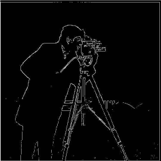
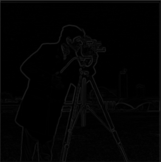
The magnitude image of the gradients is like a rough edge detection result, and we can further apply binarizing with thresholding on this image in order to suppress the noise and find real edges. We choose a threshold of 0.2 here, i.e. if a pixel in the magnitude image is greater than 0.2, then it is preserved as a part of edges and the value of it is set as 1; otherwise, it is considered not in an edge and the value is set as 0.
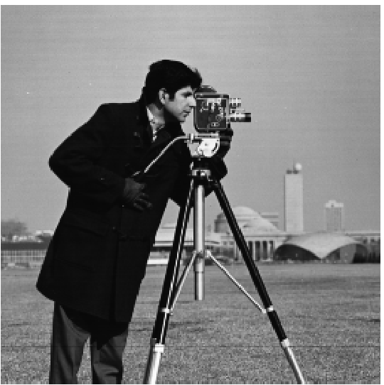
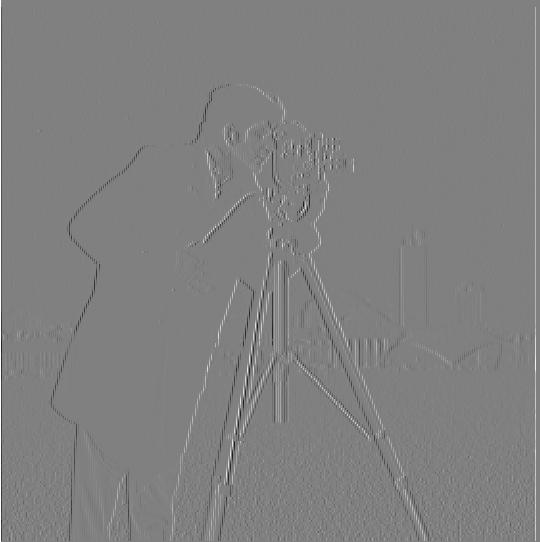
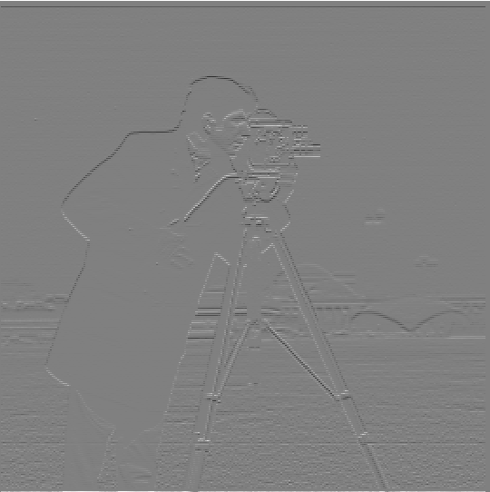
Shown below are the original image, the gradient images (normalized), the magnitude image, the binarized magnitude image.
1.2 Derivative of Gaussian (DoG) Filter
1.2.1 First Gaussian then Gradient
By applying a Gaussian filter cv2.getGaussianKernel(), i.e.
we have the blurred image
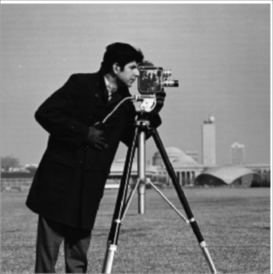
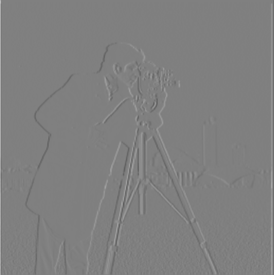
The gradient for the blurred image is
At this section and the section 1.2.2, we choose the Gaussian kernel with parameters
We do the same procedures as part 1.1, and choose a different (lower) threshold as 0.07 because the noise has been filtered through the Gaussian filter.
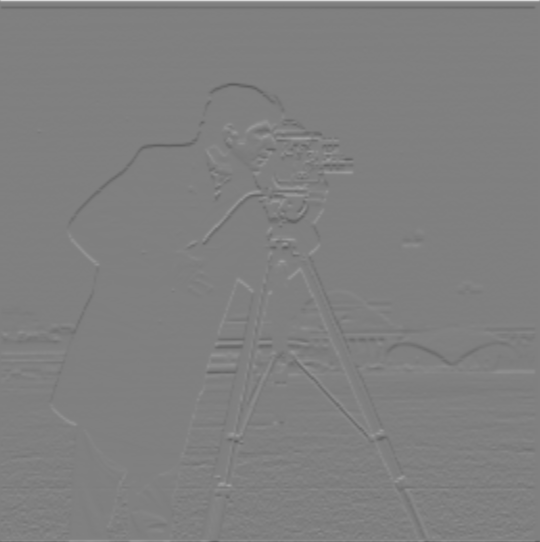
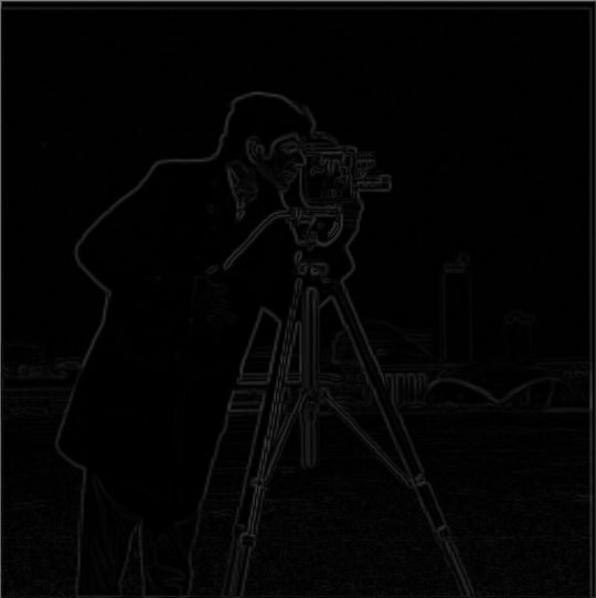

1.2.2 Derivative of Gaussian filter
We can also combine the derivative operator with the Gaussian kernel, and use the combined operators i.e. DoG filters (for two axes) to convolve the image. This is to say,
By choosing the same threshold as 1.2.1, the result is the same as above:
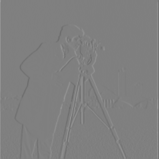
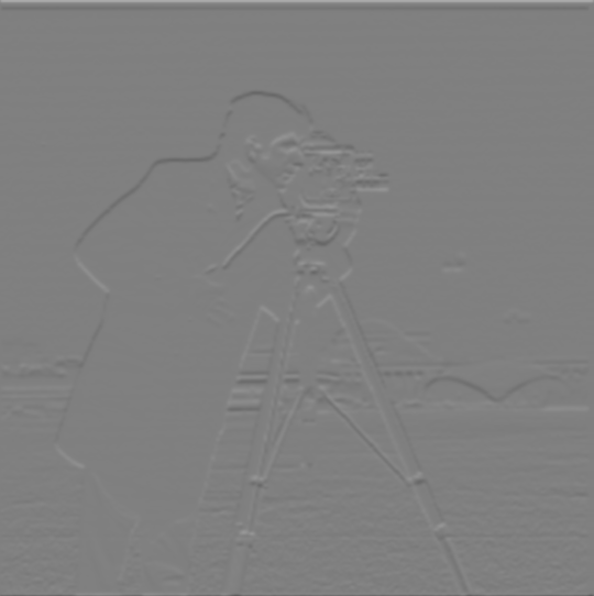

Part 2: Fun with Frequencies
2.1 Image "Sharpening"
In this section, all Gaussian filters are with the kernel same as before (the size is
2.1.1 Sharpening Progression
By adding the high frequency components with a coefficient
which means we can use one filter (called unsharp mask filter) with the expression
We choose a set of
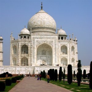


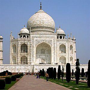

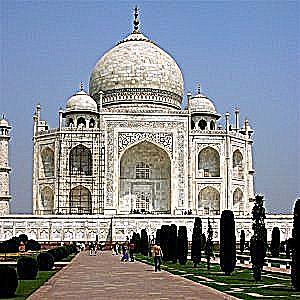
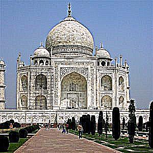
We can see the edge (patterns) of this beautiful architecture is more and more obvious in the progression when
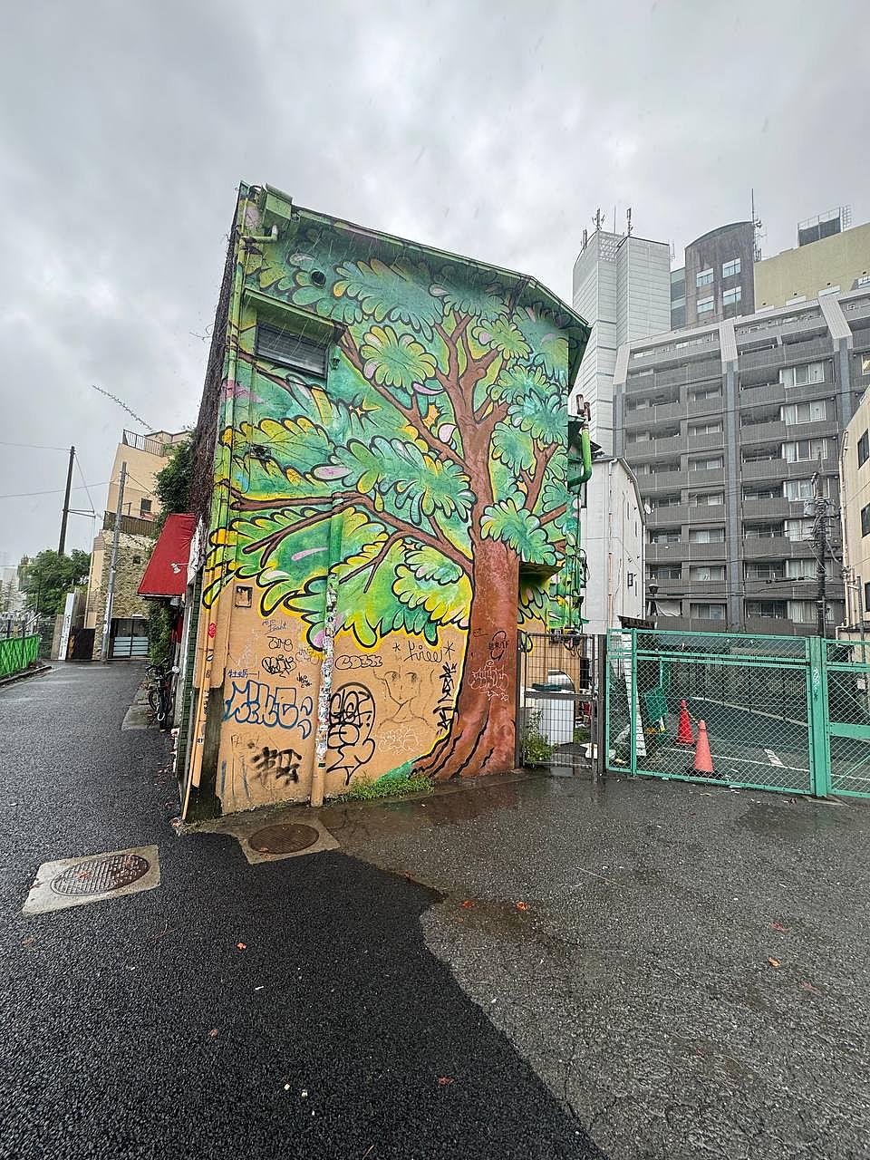
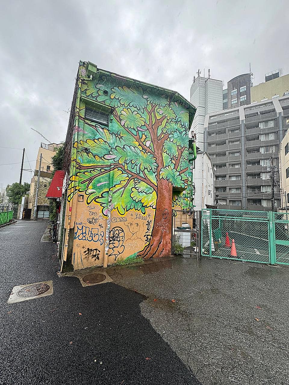
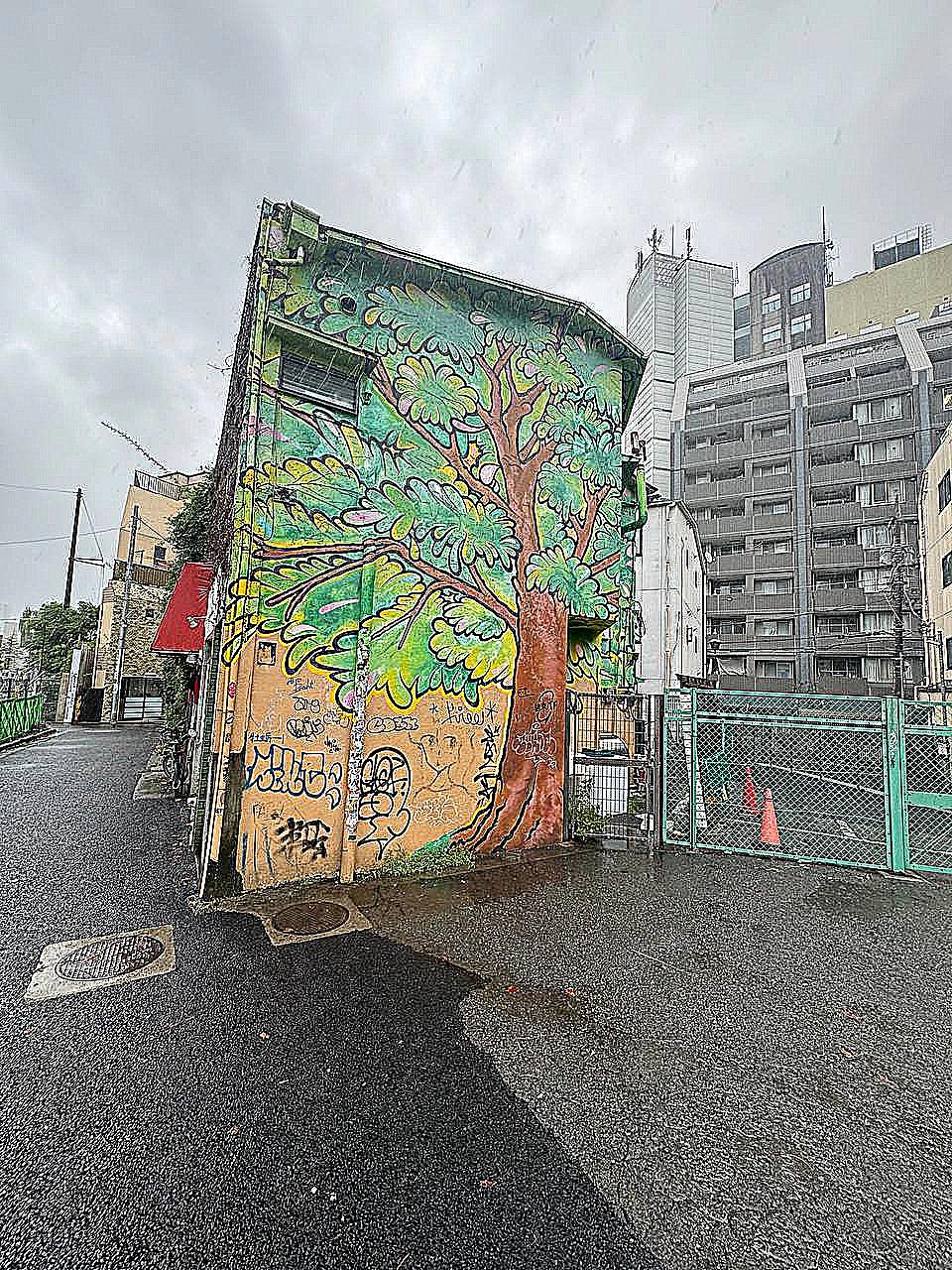
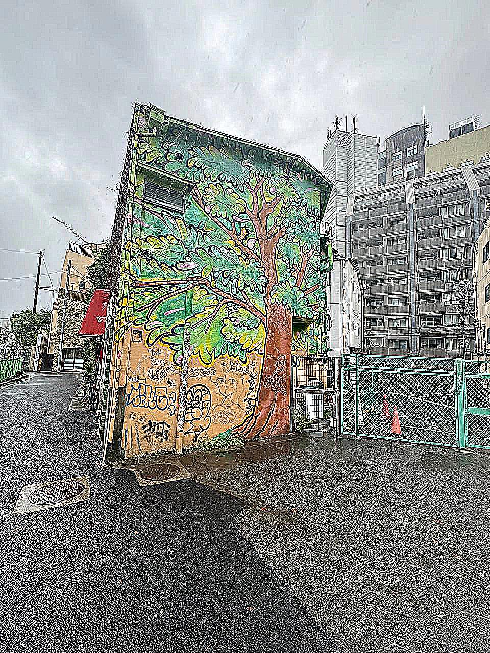
Also for my self-chosen image of a famous wall taken in Shimo-Kitazawa, Tokyo:



2.1.2 Sharpening after Blurring
For the Taj Mahal image, we try first blurring the image, then sharpen the blurred using a filter with


After being blurred, the image seems like being veiled, and re-sharpening removes this effect, but the resolution seems lower than the original, because there are some high frequency components (featuring high resolution) whose frequencies higher than the Nyquist limit in the original image is blurred by the LP filter, which is not able to be reconstruct (and also causes aliasing).
2.2 Hybrid Images
The general approach for creating a hybrid images involves these:
Align two images by rescaling, rotating and shifting;
Get the low frequency part of one image using a LP filter (we choose a Gaussian here though);
Get the low frequency of another using probably another LP filter (this could be different from that in 2), and get the high frequency part by subtracting the original image with the low frequency part. This can also be reached with a Laplacian filter.
For all cases below, we all choose a square kernel with the width/height 7 times of the sigma for each Gaussian filter.
We show two successful cases of creating hybrid images, and one failure.
2.2.1 Result 1
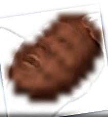
The sigma for the image for low frequency is sigma_lo=5. The other sigma is sigma_hi=3.
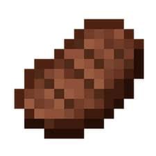
Minecraft Steak (for low frequency)
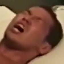
Some shouting male (for high frequency)
2.2.2 Result 2

Savoring Emoji (for low frequency)

Fearing Emoji (for high frequency)

At first sight I could see the fear, nonetheless focusing less and the joy hidden behind will emerge.
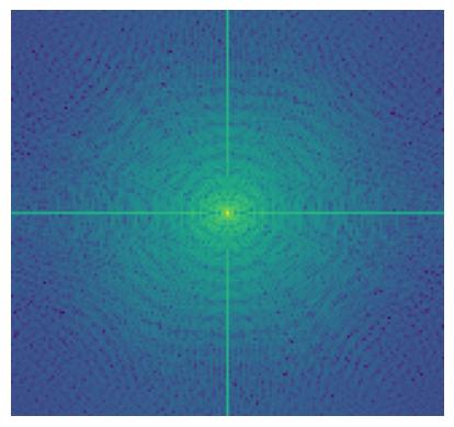
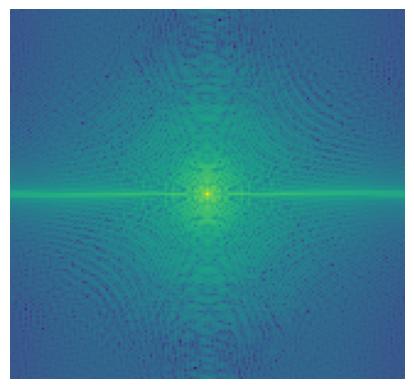
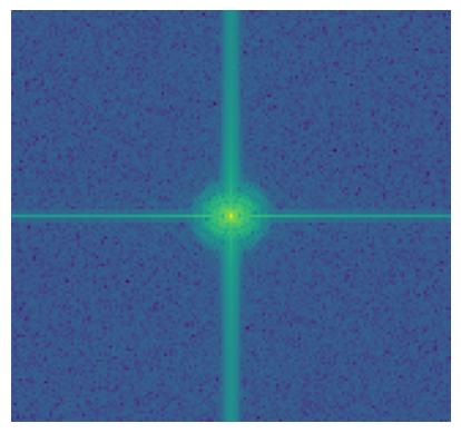
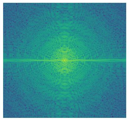
We do Fourier transform to these original (aligned), filtered images and the hybrid image.

2.2.3 Result 3 (Failed)

Exploding Cat (for low frequency)
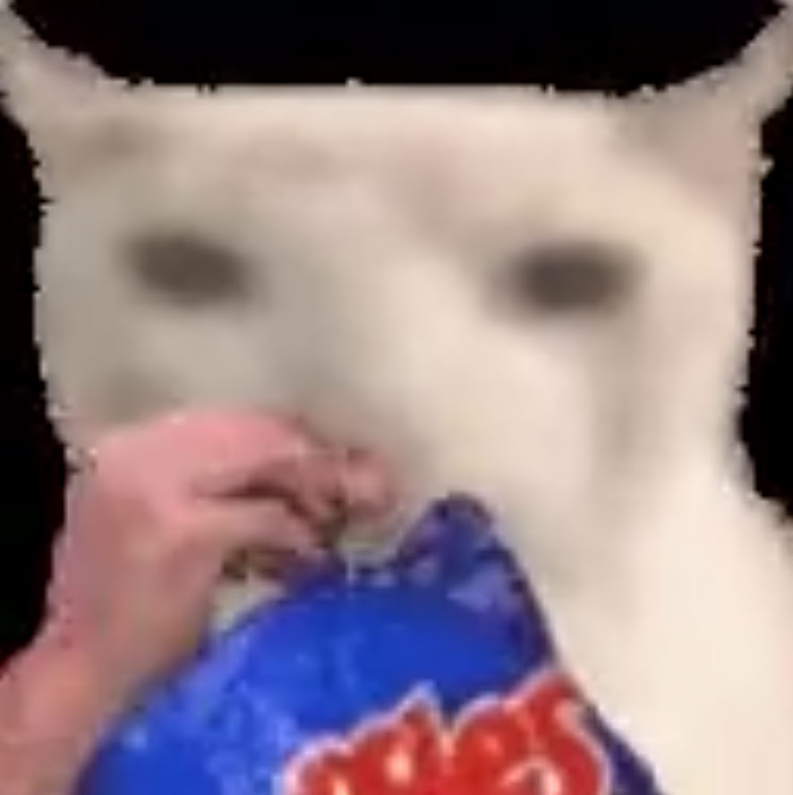
Eating Cat (for high frequency)

Though it mix well, but we could percept two features at the same time, for which I think it's a failure. I think it's because the original images are in low resolution, and the main feature (the cat) overlaps too perfectly with no other to-be-overlapped features which could make this be called a hybrid image.
2.3 Gaussian and Laplacian Stacks
In a Gaussian stack, we have the first image as the original image, and the every next image is the result of the last image in the stack convoluted with a Gaussian filter. In a Laplacian stack, every image with index i except the last one is the difference between the image i in the Gaussian stack and the next image i+1 in the Gaussian stack, and the last image is the same as the last image in the Gaussian stack which can make the whole stack adding up to the original image.
With help of the Gaussian and Laplacian stacks, we can smoothly blend the parts of two images together instead of Alpha blending (interpolating the pixel values of two images with a weight). In detail, for images A and B, we have the Gaussian stack G_A and G_B, and the Laplacian stack L_A and L_B, also the mask M (a binary image with the same size as A and B), for which we also build a Gaussian stack G_M. The blended image C is the collapsed (summed) every layer of two Laplacian stacks added together interpolated w.r.t. the mask extracted from the same layer index in G_M.
In implementation, for the Oraple we have 6-level stacks. Sigmas are always 5 and the kernel size is 7 times of that.


2.4 Multi-resolution Blending
Given the approach of blending introduced in 2.3, we could blend any pair of images with some masks. The sigma/kernel/level number settings remain from 2.3.
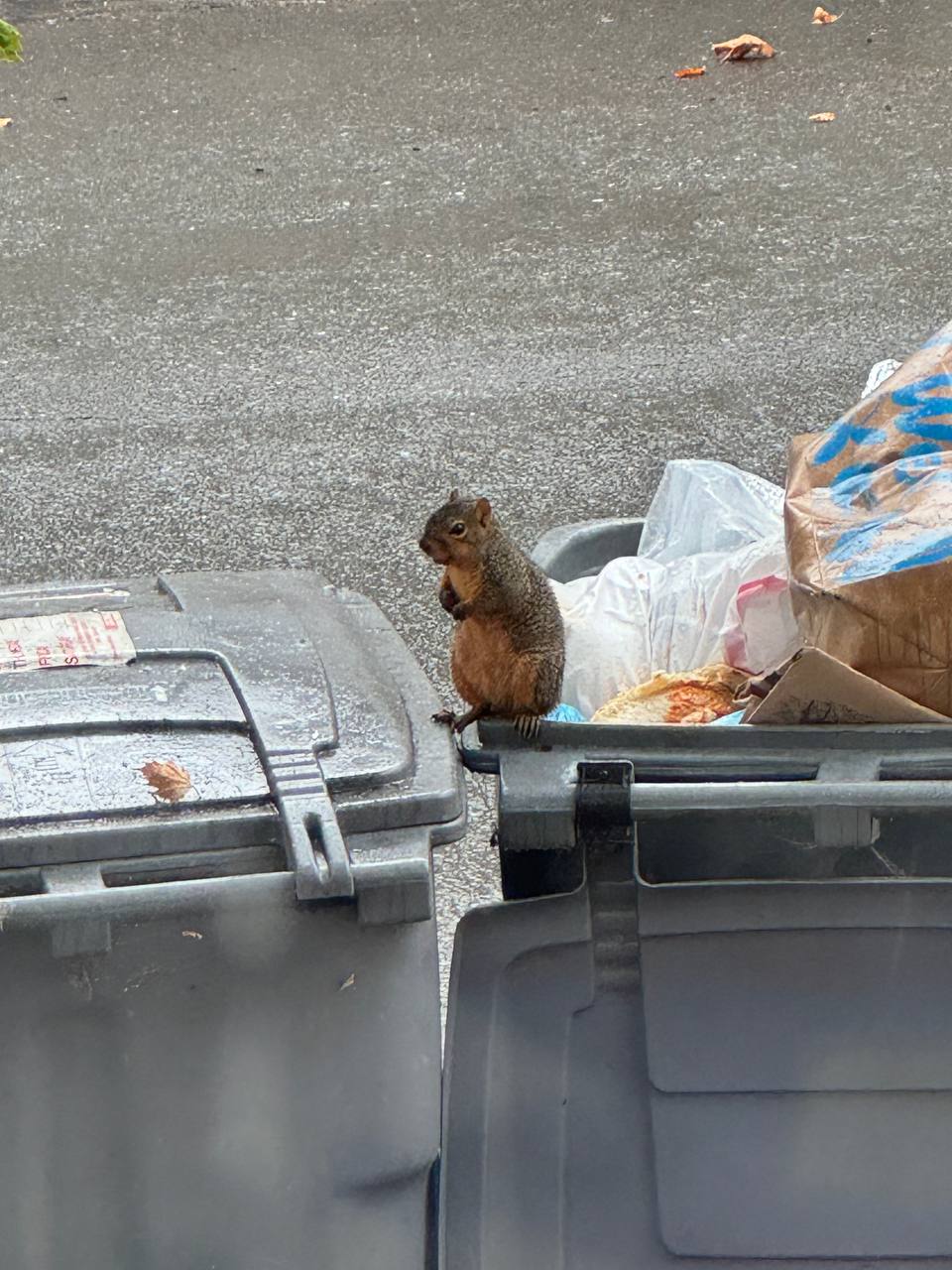
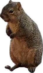
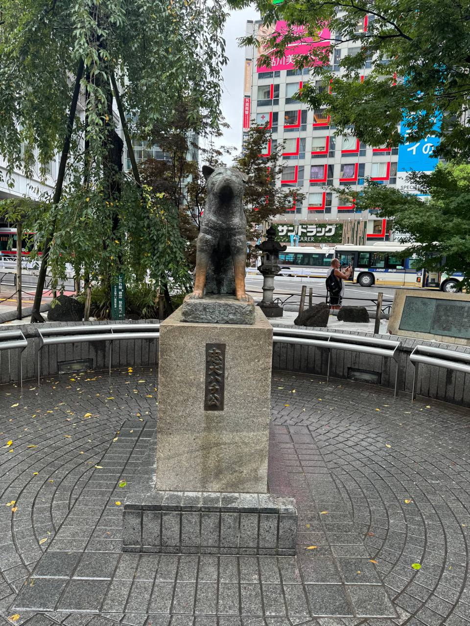
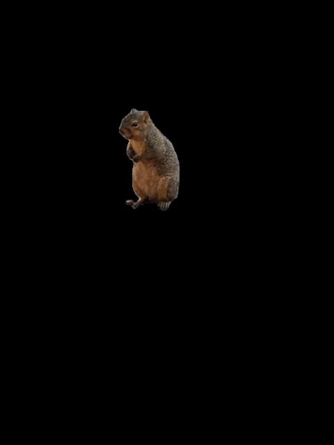
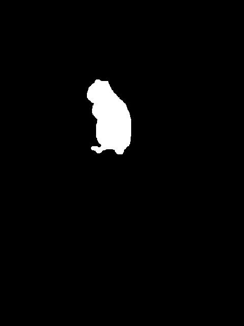
When generating masks, I used Segment-Anything by Meta to cut out an transparent-background sub-image (which is a feature) from one photo I have taken, and manipulated the shifting and resizing by hand.
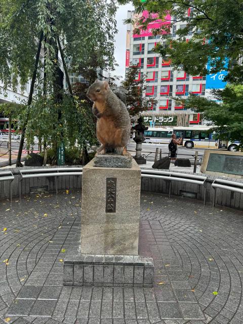
2.4.1 Statue of Hachiko the Squirrel
Sigma for the squirrel: 7
Sigma for the Hachiko statue: 13
Sigma for the Gaussian stack: 7
Kernel size: 7*sigma
Number of levels for the stacks: 8
2.4.2 Extra Chashu to My Ramen
(but only 1 piece in 2)
Sigma for every stack: 7
Kernel size: 7*sigma
Number of levels for the stacks: 8
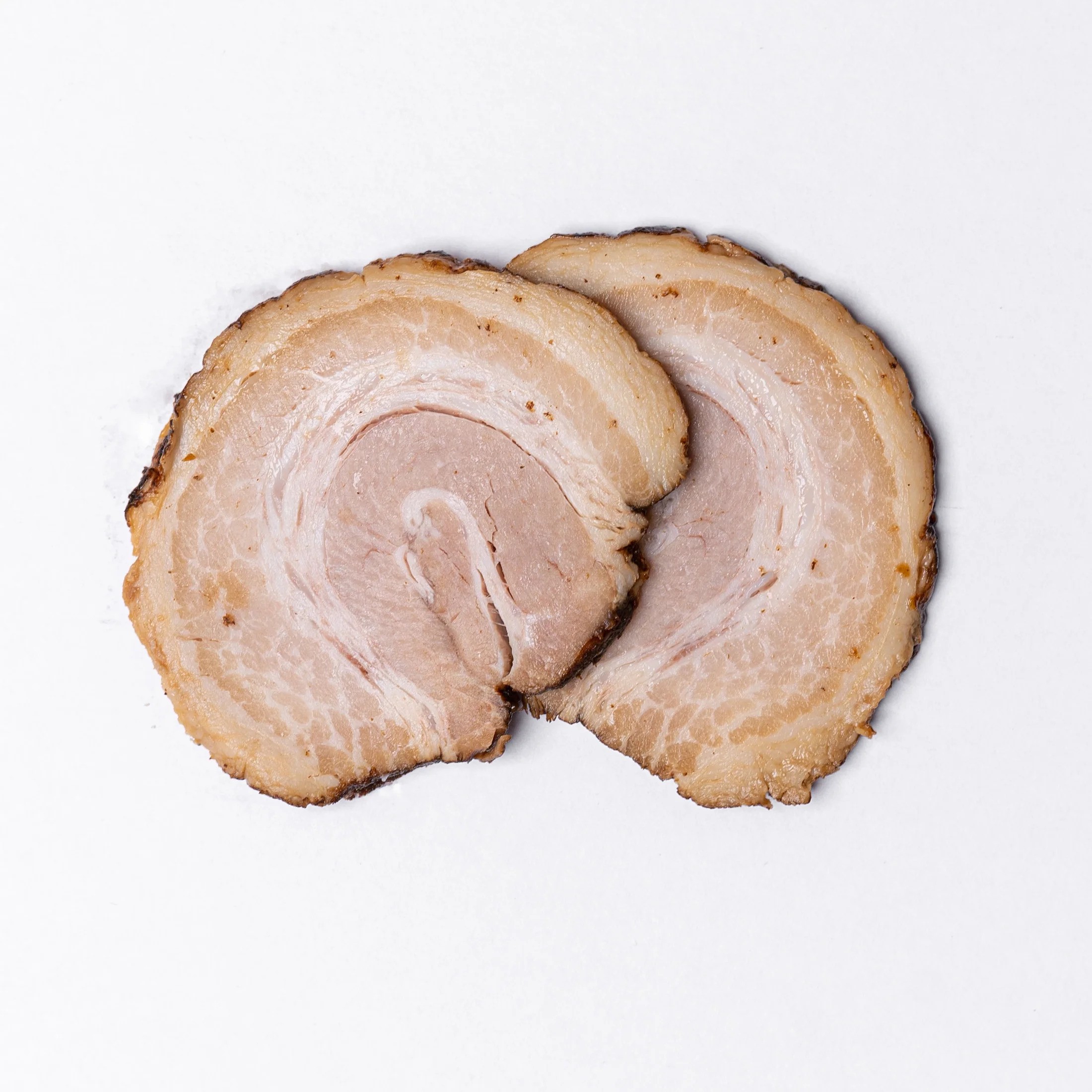
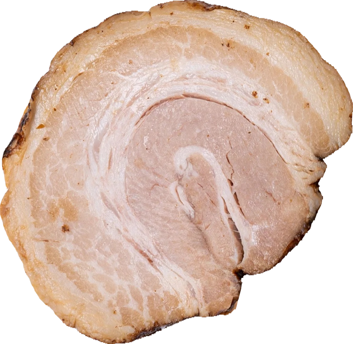
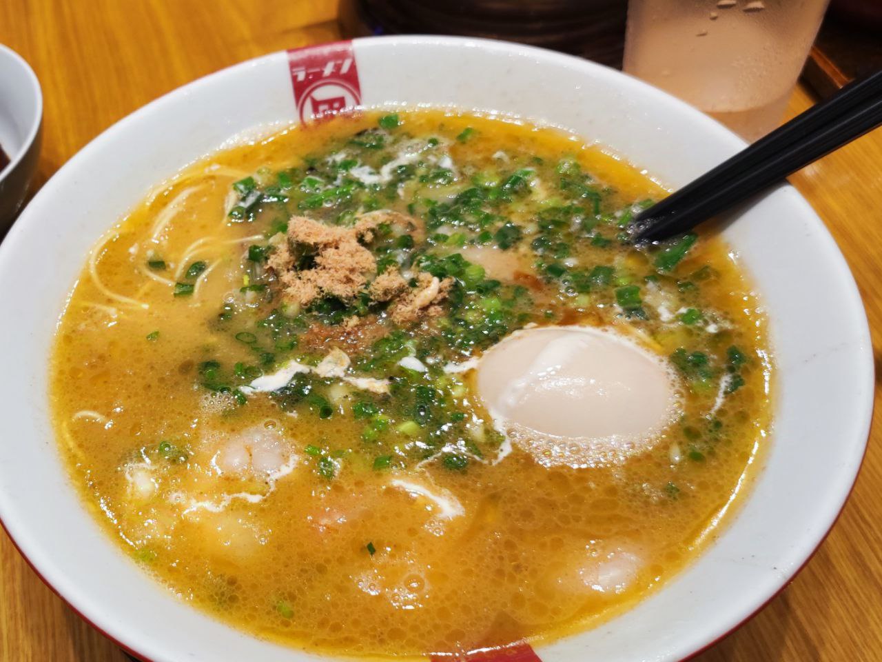
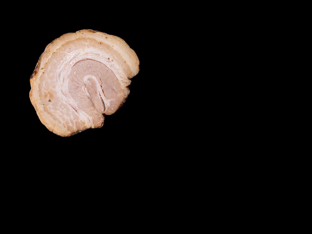
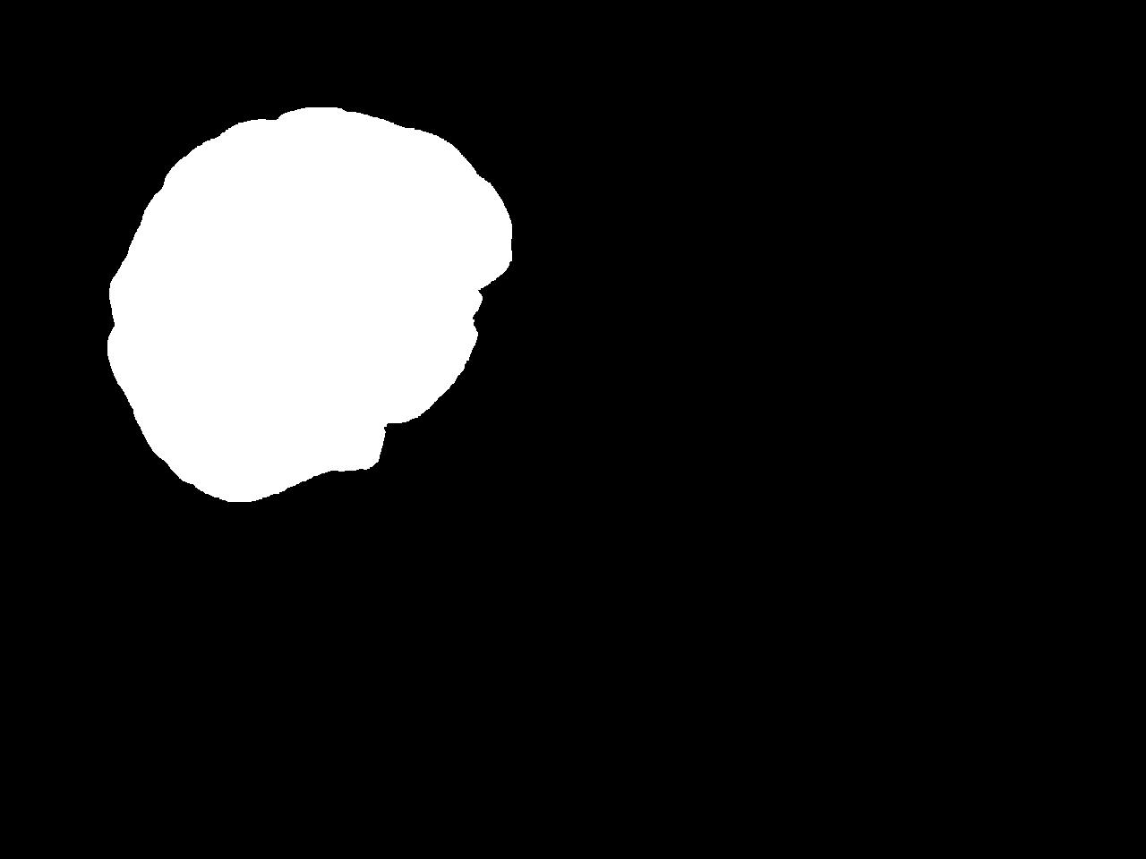
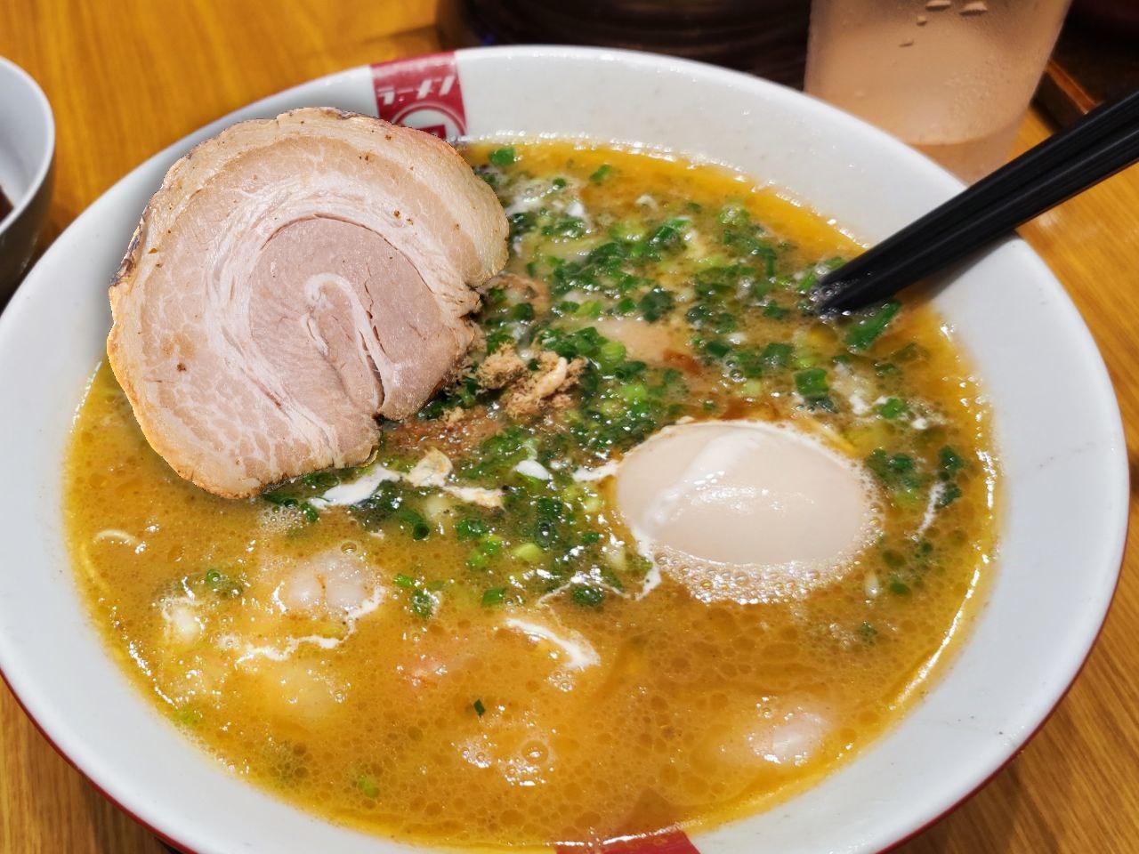
The chashu blended into the noodles seems smooth, especially for the shadow appears at the upper part (which is not in the cut-out image and the black-background image) and the lower part is colored by the soup.
The Laplacian/Gaussian Stacks before/after masking is as shown as below.


